From the Galerkin Method to the Finite Element Method

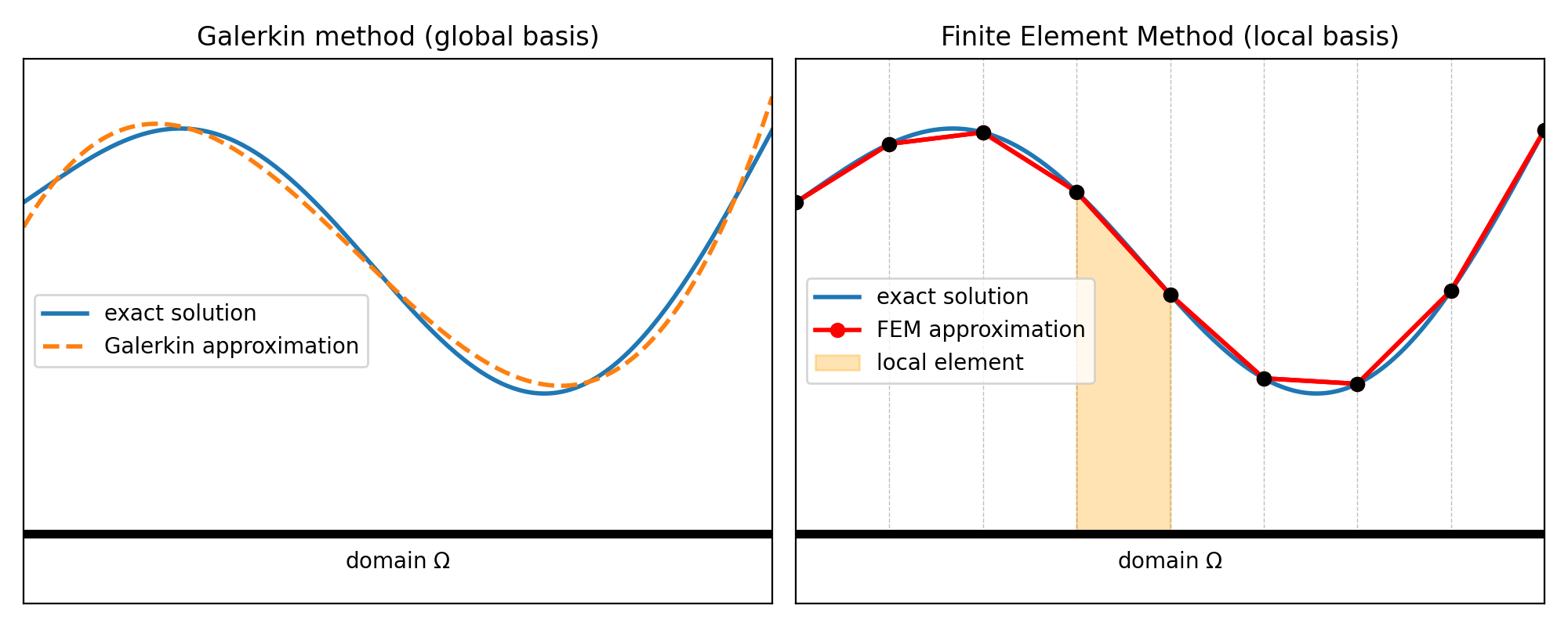
In the previous lecture, we discussed the Galerkin method, a powerful approach for finding approximate solutions to differential equations by minimizing the residual over the domain. The Finite Element Method (FEM) can be seen as a natural extension of the Galerkin method. In FEM, the domain of the problem is divided into smaller subdomains called finite elements, and on each element, we approximate the solution using simple, locally defined functions known as shape functions. By applying the Galerkin procedure element by element, we construct local equations that are then assembled into a global system describing the behavior of the entire structure. In other words, FEM is a Galerkin method applied to a discretized domain, where the flexibility of dividing the domain into elements allows us to handle complex geometries, varying material properties, and arbitrary boundary conditions. This combination of local approximation and global assembly is what makes FEM a versatile and widely used tool in engineering and applied mechanics.

Introduction to the Finite Element Method

The Finite Element Method (FEM) is one of the most popular computational methods used to solve problems in mechanics. The essence of FEM is to replace the differential equations describing a given problem with a system of algebraic equations with boundary conditions.

The Finite Element Method is carried out in the following stages division of the domain into subdomains (finite elements). This process is called discretization. The subdomains should be simple (triangle, square, cuboid)

• construction of the finite element
• assembly process
• application of boundary conditions
• solution of the system of algebraic equations
• calculation of additional quantities (deformation, stress, force)

Bar Tension

This is a one-dimensional boundary value problem in structural mechanics describing the axial deformation of a straight bar subjected to external loads.

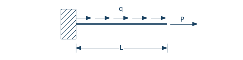
The ordinary differential equation together with the boundary conditions that describe this problem are as follows.

$$EA\cfrac{d^2u(x)}{dx^2} + q = 0$$

Boundary conditions:
• the bar is fixed at $x=0$
• axial force at the free end $x=L$

$$u(x=0) = 0, \qquad EA\cfrac{du(x=L)}{dx} = P$$

Domain:

$$\Omega = (0, L), \qquad 0 \leq x \leq L$$

Where:
• $u(x)$ — axial displacement of the bar
• $E$ — Young’s modulus of the material
• $A$ — cross-sectional area of the bar
• $q$ — distributed axial load (force per unit length)
• $P$ — concentrated force applied at the free end
• $L$ — length of the bar

Discretization of the Bar

Let us divide our domain $\Omega$ into subdomains, which we will call finite elements. Assume that the domain $\Omega$, contained between points $a$ and $b$, where $a \leq x \leq b$, is divided into $n$ subdomains (elements), as shown in the figure. Let us denote by $\Omega^{e}$, where $e$ varies from $1$ to $n$, the region occupied by a single finite element. The points defining the division into finite elements will be called nodes. The collection of all finite elements will be called the finite element mesh.

$$\Omega = \Omega^1 \cup \Omega^2 \cup ... \cup \Omega^n.$$

Each element is bounded by two nodes. The total number of nodes in the considered case is $N+1$.

Equations Describing a Finite Element

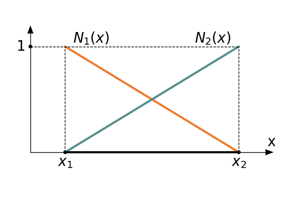
Let us analyze a two-node element with nodes at points $x_1$ and $x_2$. Assume that within the element, the variation of the unknown field is described by the relation

$$u(x) = u_1 N_1(x)+ u_2 N_2(x)$$

where the shape functions $N_1$ and $N_2$ have the form

$$N_1 = \cfrac{x_2-x}{x_2-x_1}, \qquad N_2 = \cfrac{x-x_1}{x_2-x_1}$$

The parameters $u_1$ and $u_2$ are the unknown nodal displacements.

The solution on the element can be written in matrix form as

$$u(x) = \N\u, \quad \N = [ N_1, N_2], \quad \u = [u_1, u_2]^T$$

The vector $\mathbf{u}$ is a column vector so that matrix multiplication (dot product) can be performed. The two-component matrix $\N$ collects the shape functions. The vector $\u$ contains the unknown nodal displacements. We substitute our approximate solution into the differential equation. In the next step, we multiply the equation by $\N^T$ and integrate over the domain of the considered finite element.

$$EA\cfrac{d^2}{dx^2}\mathbf{N}\mathbf{u} + q(x) = 0 \qquad |\int_{x_1}^{x_2} \cdot \mathbf{N}^T$$

In the Galerkin method, the residual is minimized by multiplying the equation by a test function and integrating over the domain, i.e.

$$\int_{x_1}^{x_2} \mathbf{N}^TEA\cfrac{d^2\mathbf{N}}{dx^2}\mathbf{u} dx + \int_{x_1}^{x_2}\mathbf{N}^Tq(x) dx = 0$$

The above expression means that we obtain two equations because we have two shape functions. That is why we multiply by $\N^T$—otherwise, we would not obtain two equations. The number of equations must equal the number of shape functions in the element.

Let us apply integration by parts and multiply by -1:

---

$$\int f(x) \cdot g{'}(x) dx = f(x) \cdot g(x) - \int f{'}(x) \cdot g(x) dx$$

---

i.e. $f(x) = \mathbf{N}^T, \, g(x) = \cfrac{d \N}{dx}$

$$\int_{x_1}^{x_2} EA \cfrac{d\mathbf{N}^T}{dx}\cfrac{d\mathbf{N}}{dx} dx\mathbf{u}-\int_{x_1}^{x_2} \mathbf{N}^T q(x) dx - EA\mathbf{N}^T\cfrac{d\mathbf{N}}{dx}\mathbf{u}|_{x=x_2} + EA\mathbf{N}^T\cfrac{d\mathbf{N}}{dx}\mathbf{u}|_{x=x_1}=0$$

The above equation is called the weak (variational) formulation. The term “weak” refers to the fact that the differentiability requirements for the displacement function $u(x)$ are reduced. Let us rewrite the above equation using the following notation

$$\k = \int_{x_1}^{x_2} EA \cfrac{ d\mathbf{N}^T}{dx} \cfrac{d\mathbf{N}}{dx} dx$$ $$\mathbf{f}_{\mathbf{2\times 2}} = \int_{x_1}^{x_2} \mathbf{N}^T q(x) dx$$ $$\mathbf{Q}_{\mathbf{2\times 2}} = EA\mathbf{N}^T\cfrac{d\mathbf{N}}{dx}\mathbf{u}|_{x=x_2} - EA\mathbf{N}^T\cfrac{d\mathbf{N}}{dx}\mathbf{u}|_{x=x_1}$$ $$\k_{\mathbf{2\times 2}} \mathbf{u_{2\times 1}} = \mathbf{f}_{\mathbf{2\times 1}} + \mathbf{Q}_{\mathbf{2\times 1}}$$

Let us now consider the first integral (the local stiffness matrix of the finite element). Let the length of the element be denoted by $L$

$$k_{11} = \int_{x_1}^{x_2} EA \cfrac{dN_1}{dx}\cfrac{dN_1}{dx} dx = EA\int_{x_1}^{x_2} -\cfrac{1}{x_2-x_1} \cdot \left(-\cfrac{1}{x_2-x_1}\right) dx =$$ $$k_{11} = EA \cfrac{x}{(x_2-x_1)^2}|_{x_1}^{x_2} = EA \left(\cfrac{x_2}{(x_2-x_1)^2}- \cfrac{x_1}{(x_2-x_1)^2}\right) = EA \cfrac{x_2-x_1}{(x_2-x_1)^2} = \cfrac{EA}{x_2-x_1} = \cfrac{EA}{L}$$ $$k_{12} = -\cfrac{EA}{L}$$

where $L$ is the length of the considered finite element.

$$\k_{\mathbf{2\times 2}} = \cfrac{EA}{L^e} \matt{1}{-1}{-1}{1}$$

Now let us consider the second integral, i.e. $\f$

$$f_1 = \int_{x_1}^{x_2} N_1(x) q dx = \cfrac{1}{2}qL, \qquad f_2 = \int_{x_1}^{x_2} N_2(x) q dx = \cfrac{1}{2}qL$$

Using matrix notation, we obtain

$$\mathbf{f}_{\mathbf{2\times 1}} = \cfrac{1}{2}qL^e\vcc{1}{1}$$

Let us now consider the nodal force vector, introducing the notation

$$Q_2 = EA\cfrac{d\mathbf{N}}{dx}\u|_{x=x_2}, \qquad Q_1 =-EA\cfrac{d\mathbf{N}}{dx}\u|_{x=x_1}$$

Thus we have

$$= \mathbf{N}^T(x_2)Q_2 + \mathbf{N}^T(x_1)Q_1 = \vcc{0}{1}Q_2 + \vcc{1}{0}Q_1 =\vcc{Q_1}{Q_2}$$

• $\k$ - symetryczna macierz kwadratowa (macierz sztywności elementu skończonego
• $\u$ - wektor kolumnowy przemieszczeń węzłowych elementu
• $\f$ - wektor kolumnowy obciążeń ciągłych elementu
• $\Q$ - wektor kolumnowy sił węzłowych elementu.

Assembly of Finite Elements

So far, our discussion has focused on a single finite element. Let us now divide our structure into $n$ finite elements. Consider two neighboring elements $\Omega^e$ and $\Omega^{e+1}$.

• Continuity conditions of displacements at the nodes

$$u_2^e = u_1^{e+1}$$

• Equilibrium conditions of forces at the nodes

$$Q_2^e + Q_1^{e+1} = 0$$

If an external force is applied at the node, then

$$Q_2^e + Q_1^{e+1} = P$$

Note: If concentrated loads appear along the length of the bar, we must insert nodes at those points to account for them.

Let us now introduce a global numbering of nodal displacements.

$$u_1^1 = U_1, \quad u_2^1 = u_1^2 = U_2, \quad u_2^2 = u_1^3 = U_3, ..., \quad u_2^{N-1} = u_1^N = U_N, \quad u_2^N = U_{N+1}$$

Let us write out the equations for the elements using the new global notation:
• 1) $k_{11}^1 U_1 + k_{12}^1U_2 = f_1^1 + Q_1^1$
• 2) $k_{21}^1 U_1 + k_{22}^1U_2 = f_2^1 + Q_2^1$
• 3) $k_{11}^2 U_2 + k_{12}^2 U_3 = f_1^2 + Q_1^2$
• 4) $k_{21}^2 U_2 + k_{22}^2U_3 = f_2^2 + Q_2^2$
• $\vdots$

• 2N) $k_{21}^N U_N + k_{22}^NU_{N+1} = f_2^N + Q_2^N$

Using the equilibrium conditions, we can combine equation 2) with equation 3). The first and last equations remain unchanged. The total number of equations then becomes $1 + 1 + (2n-2)/2 = n+1$.

• 1) $\quad k_{11}^1 U_1 + k_{12}^1U_2 = f_1^1 + Q_1^1 \quad \text{unchanged}$
• 2) $\quad k_{21}^1 U_1 + k_{22}^1U_2 \quad k_{11}^2 U_2 + k_{12}^2 U_3 = f_2^1 + Q_2^1 + f_1^2 + Q_1^2$
• 3) $\quad k_{21}^1 U_1 + k_{22}^1U_2 \quad k_{11}^2 U_2 + k_{12}^2 U_3 = f_2^1 + Q_2^1 + f_1^2 + Q_1^2$
• 4) $\quad k_{21}^1 U_1 + (k_{22}^1 \quad k_{11}^2) U_2 + k_{12}^2 U_3 = f_2^1 + Q_2^1 + f_1^2 + Q_1^2$
• N+1) $\quad k_{21}^N U_N + k_{22}^NU_{N+1} = f_2^N + Q_2^N \quad \text{unchanged}$

This system of linear equations can be written in matrix form as:

$$\begin{bmatrix} k_{11}^1 & k_{12}^1 & 0 & 0 & \ldots & 0 \\k_{21}^1 & k_{22}^1+k_{11}^2 & k_{12}^2 & 0 & \ldots & 0 \\ E0 & k_{21}^2 & k_{22}^2+k_{11}^3 & & \ldots & 0 \\ \vdots & \vdots & \vdots & \vdots & \ddots & \vdots \\ 0 & 0 & 0 & 0 & \ldots & k_{22}^N \\\end{bmatrix}\begin{bmatrix} U_1 \\U_2\\ U_3\\ \vdots \\ U_{n+1}\\\end{bmatrix}=\begin{bmatrix} f_1^1 \\f_2^1+f_1^2\\ f_2^2+f_1^3 \\ \vdots \\ f_2^N\\\end{bmatrix}\begin{bmatrix} Q_1^1 \\Q_2^1+Q_1^2\\ Q_2^2+Q_1^3 \\ \vdots \\ Q_2^N\\\end{bmatrix}$$

Or, more compactly:

$$\K \mathbf{U} = \mathbf{F}$$