Applied Continuum Mechanics with Abaqus

Introduction

Postprocessing in Abaqus refers to the analysis and interpretation of simulation results after the simulation has been completed. Abaqus provides a range of tools and features for postprocessing to help users visualize and understand the behavior of their models.

Abaqus/CAE visualization module

The primary purpose of Abaqus visualization module is to provide a graphical interface for visualizing and interpreting simulation results. It offers a variety of tools and options for displaying different types of results, such as contour plots, deformed shape plots, vector plots, and more.

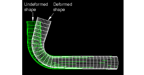
Odb icons: Undeformed shape, Deformed shape, Contours, Symbols, Material orientations, X–Y data, Time history animation, Scale factor animation, Harmonic animation.

Undeformed shape
An undeformed shape plot displays the initial shape or the base state of your model.

$$\x(\X,t) = \X$$

Deformed shape
A deformed shape plot displays the shape of your model according to the values of a nodal variable such as displacement.

$$\x(\X,t) = \X + \u(\X,t)$$

Deformed shape superimposed on the undeformed shape.

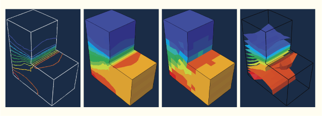
Contours
A contour plot displays the values of an analysis variable such as stress or strain at a specified step and frame of your analysis. Abaqus/CAE represents the values as customized colored lines, colored bands, colored faces, colored isosurfaces, or tick marks on the model.

$$\sigma_{11}(\x,t), \quad \sigma_{11}(\X,t)$$

From left to right: contours shown as colored lines, colored bands, colored faces, and colored isosurfaces.

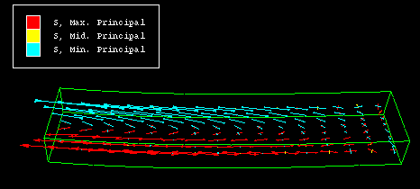
Symbols
For an output database, a symbol plot displays the magnitude and direction of a particular vector or tensor variable at a specified step and frame of your analysis.

$$\v(\x,t), \quad \v(\X,t)$$

Symbol plot of principal stress.

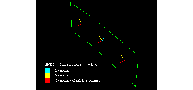
Material orientations
A material orientation plot displays the material directions of elements in your model at a specified step and frame of your analysis. The Visualization module represents the material directions as material orientation triads at the element integration points.

$$\F = \R\U \rightarrow \R(\x,t)$$

Material orientation plot.

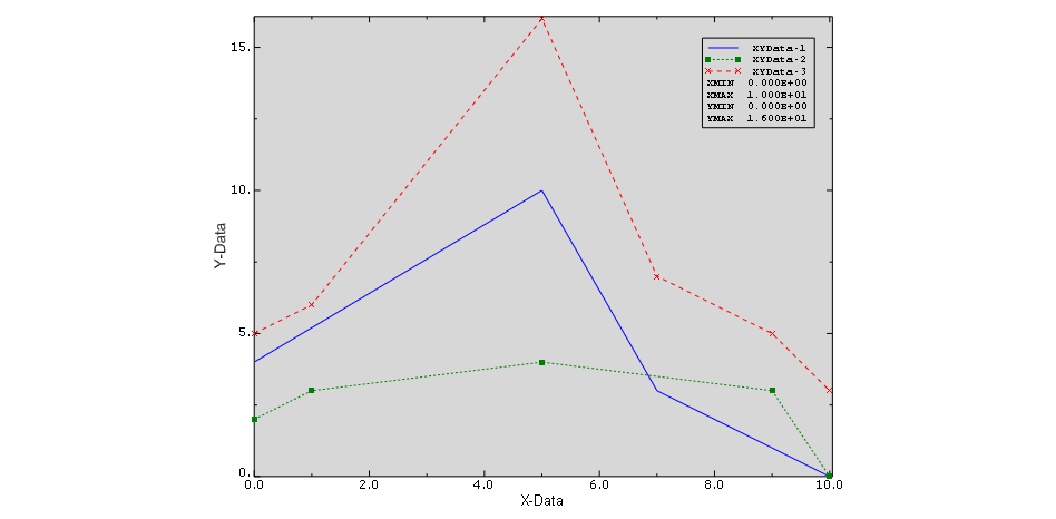
X–Y data
An X–Y plot is a two-dimensional graph of one variable versus another.

$$\sigma_{11}(\X_0,t), \quad \varepsilon_{11}(\X_0,t)$$

X–Y plot displaying three objects of data.

Time history animation
Time history animation displays a series of plots in rapid succession, giving a movie-like effect. The individual plots vary according to actual result values over time.

$$p(\x,t_i) \quad t_i = t_1, t_2, \ldots, \t_n$$

Scale factor animation
Scale factor animation displays a series of plots in rapid succession, giving a movie-like effect. The individual plots vary in the scale factor applied to a particular deformation. Abaqus/CAE generates animation scale factors ranging from 0 to 1 or from –1 to 1.

$$\x(\X,t) = \X + s_i\u(\X,t), \quad \quad s_i = s_1, s_2, \ldots, \s_n$$

Harmonic animation
Harmonic animation displays a series of plots in rapid succession, giving a movie-like effect. The individual plots vary according to the angle applied to the complex number results being displayed.

Probing models, model plots, and X–Y plots
Probing displays model data and analysis results as you move the cursor around a model or a model plot; probing an X–Y plot displays the coordinates of graph points. You can write this information to a file.

Additional capabilities

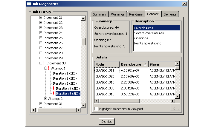
Visualizing diagnostic information

Diagnostic information helps you determine the causes of nonconvergence in a model. You can view information for each stage of the analysis and use Abaqus/CAE to highlight problematic areas on the model in the viewport.

The Job Diagnostics dialog box.

Generating tabular data reports
Abaqus allows to produce a tabular data report of X–Y data objects, field output results, probe values, or free body cuts. Abaqus/CAE writes the report to the file name of your choice. Generate a tabular report to save data values beyond the duration of the session or to print these values.

Visualisation module -> menu -> Report

Output variable identifiers

• U - displacement vector
• V - velocity vector
• A - acceleration vector
• Rf - reaction force vector

• S - true Cauchy stress tensor
• MISES - Mises equivalent stress, defined as

$$q=\sqrt{\cfrac32 S_{ij}S_{ij}}, \quad \text{where} \quad S_{ij} \quad \text{is deviatoric stress tensor}$$

• PRESS - pressure stress,

$$p=-\cfrac13 \tr(\ss)$$

• TRESC - Tresca equivalent stress, defined as the maximum difference between principal stresses.
• INV3 - Third stress invariant, defined as

$$r = \left(\cfrac92 S_{ij} S_{jk} S_{ki} \right)^{1/3}$$

• E - small strain tensor
• LE - logarithmic strain tensor
• EE - elastic strain tensor
• PE - plastic strain tensor
• PEEQ - equivalent plastic strain

$$\dot{\bar{\ee}}^{pl} = \sqrt{\cfrac23 \dot{\ee}^{pl} \cdot \dot{\ee}^{pl}}, \quad \bar{\ee}^{pl} = \int_0^t \dot{\bar{\ee}}^{pl} dt$$

• PEMAG - plastic strain magnitud,

$$\sqrt{\cfrac23 \ee^{pl} \cdot \ee^{pl}}$$

• AC YIELD - yes/no flag (1/0 on the output database) telling if the material is currently yielding or not

Accessing an output database

In Abaqus, you can use Python scripting to access and extract data from the output database (ODB) files.

The output database object model.

The openOdb method opens an existing output database. For example, the following statement opens the output database

odb = openOdb(path='path/to/your/odb/file.odb')

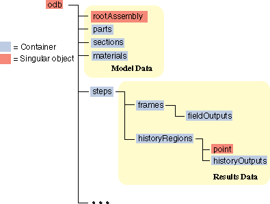
Reading model data

An output database contains only one root assembly. You access the root assembly through the OdbAssembly object.

myAssembly = odb.rootAssembly

Part instances are stored in the instances repository under the OdbAssembly object. The following statements display the repository keys of the part instances:

for instanceName in odb.rootAssembly.instances.keys():
  print(instanceName)

Regions in the output database are OdbSet objects. Regions refer to the part and assembly sets stored in the output database. A part set refers to elements or nodes in an individual part and appears in each instance of the part in the assembly. An assembly set refers to the elements or nodes in part instances in the assembly. A region can be one of the following:
• A node set
• An element set
• A surface

For example, the following statement displays the node set and element set in the OdbAssembly object:

odb.rootAssembly.nodeSets["TOP"]
odb.rootAssembly.elementSets["TOP"]

The following statements display the node sets and the element sets in the PART-1-1 part instance:

nset = odb.rootAssembly.instances['PART-1-1'].nodeSets["TOP"]
eset = odb.rootAssembly.instances['PART-1-1'].elementSets["TOP"]
for node in nset.nodes:
  print(node.label)
  print(node.coordinates)
for element in eset.elements:
  print(element.connectivity)

Reading results data

The following list describes the objects in results data and the commands you use to read results data. As with model data you will find it useful to use the keys() method to determine the keys of the results data repositories.

Steps are stored in the steps repository under the Odb object. The key to the steps repository is the name of the step. The following statements print out the keys of each step in the repository:

for step_name in odb.steps.keys():
  print(step_name)

Each step contains a sequence of frames, where each increment of the analysis (or each mode in an eigenvalue analysis) that resulted in output to the output database is called a frame. The following statement assigns a variable to the last frame in the first step:

lastFrame = odb.steps['Step-1'].frames[-1]

Reading field output data

displacement=lastFrame.fieldOutputs['U']
fieldValues=displacement.values
# For each displacement value, print the nodeLabel
# and data members.
for v in fieldValues:
    print('Node = %d u[x] = %6.4f, u[y] = %6.4f').format(v.nodeLabel, v.data[0], v.data[1])

Using regions to read a subset of field output data

center = odb.rootAssembly.instances['PART-1-1'].nodeSets['TOP']
centerDisplacement = displacement.getSubset(region=center)
centerValues = centerDisplacement.values
for v in centerValues:
    print(v.nodeLabel, v.data)

Example

Post-processing of results from lecture 04.

The developed example script can be downloaded at: