Introduction
In the context of Abaqus, a "step" refers to a specific stage of an analysis. An analysis in Abaqus is typically divided into one or more steps, where each step represents a different loading or boundary condition applied to the model.
There are several types of steps in Abaqus, including:
• Static Step: In a static step, the loads are applied gradually, and the equilibrium equations are solved at each load increment until the final load is reached.
• Dynamic Step: Dynamic analysis involves studying the response of a structure to dynamic loads, such as vibrations or impact. Dynamic steps consider the effects of time on the behavior of the system.
• Heat Transfer Step: Abaqus also allows for thermal analysis. Heat transfer steps are used to model the temperature distribution in a system.
• Eigenmode Step: Eigenmode analysis is used to determine the natural frequencies and mode shapes of a structure.
Any real problem will usually consist of more than one step during a simulation. This might consist of a loading step or a step where we apply boundary conditions.
Sometimes, we use a step in Abaqus to define different phases of loading. An example would be the simulation of a simple bow and arrow:
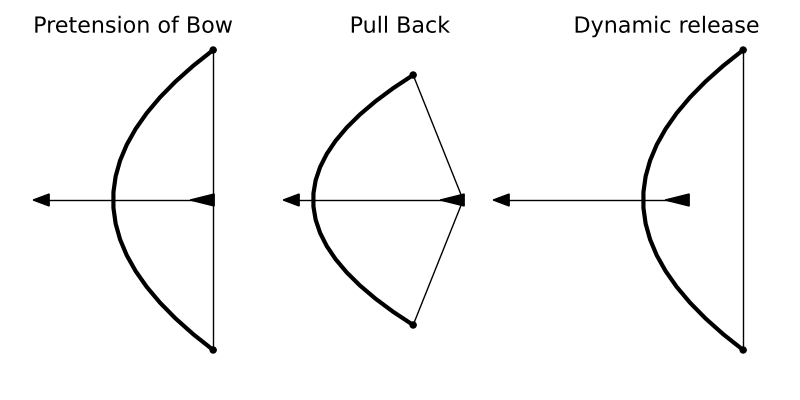
Step 1 Attaching the bowstring to pre-tension the bow.
Step 2 Pulling back the string with an arrow, storing more strain energy in the system.
Step 3
Releasing the tension on the bowstring in Step 2 converts the stored strain energy within the system into kinetic energy of the arrow.
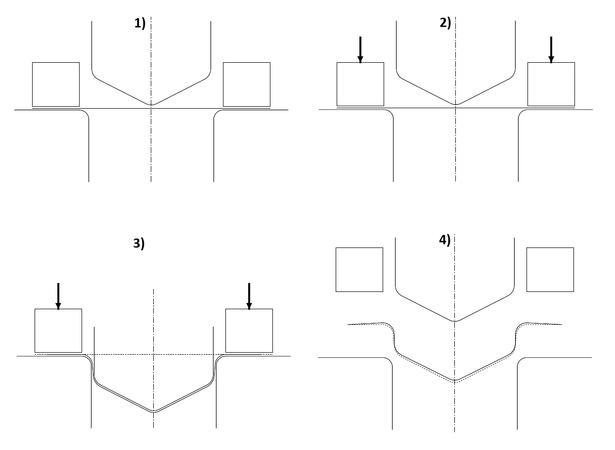
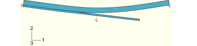
The sink is formed from sheet steel using a punch, a die, and a blank holder. This forming simulation will consist of a number of steps:
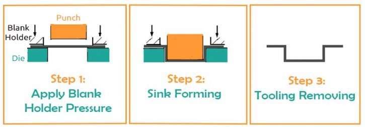
Step 1 the application of blank holder pressure
Step 2 simulating the punching operation
Step 3 the removal of the tooling, allowing the sink to spring back into its final shape
Initial and Analysis steps
Abaqus creates a special initial step at the beginning of the model's step sequence and names it Initial. It cannot be renamed, edited, replaced, copied, or deleted.
The initial step allows to define boundary conditions, predefined fields, and interactions that are applicable at the very beginning of the analysis.

For example, if a boundary condition or interaction is applied throughout the analysis, it is usually convenient to apply such conditions in the initial step.
General vs Linear Perturbation step
General step is meant to be used whenever nonlinearities occur. Each general step uses the state of the model from the previous general step so that the model is subjected to continuous evolution following specified load history.
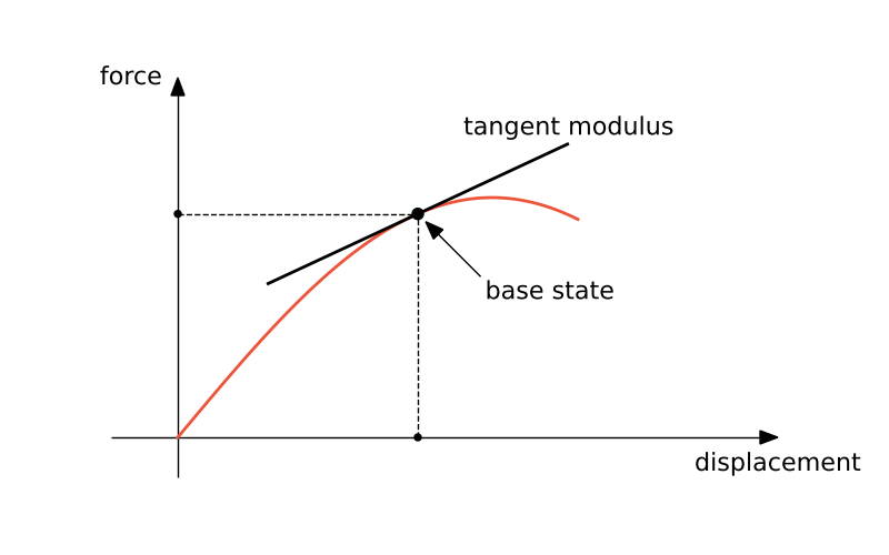
Linear perturbation steps assume linear perturbation response about so-called base state (state of the model obtained from last general step before linear perturbation step or from initial conditions).
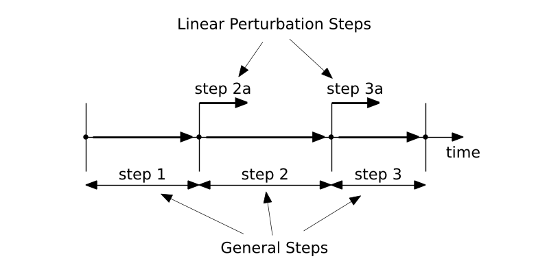
As the name suggests, in the case of this step nonlinearities can't be included. Typically, these simulations are used to obtain eigenfrequencies of the system.
The general static step may be replaced with a linear perturbation one if there is a need to enforce linearity of analysis.
Perturbation steps
Linear perturbation procedures are available only in Abaqus/Standard.
Static, linear perturbation
The base state is the current state of the model at the end of the last general analysis step prior to the linear perturbation step. If the first step of an analysis is a perturbation step, the base state is determined from the initial conditions.
If the general analysis includes a contact, its status is frozen.
Frequency
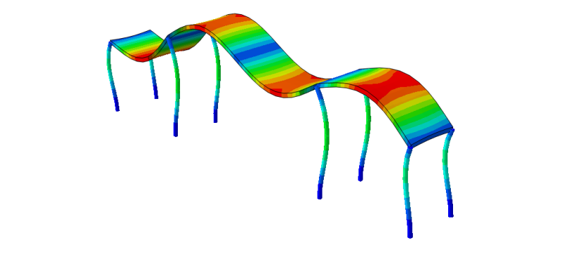
The frequency extraction procedure performs eigenvalue extraction to calculate the natural frequencies and the corresponding mode shapes of a system.
The eigenvalue problem for the natural frequencies is defined as
$$(-\omega^2 \M + \K)\boldsymbol{\phi}=0$$where $\M$ is the mass matrix (which is symmetric and positive definite), $\K$ is the stiffness matrix (which includes initial stiffness effects if the base state included the effects of nonlinear geometry), $\omega$ is the circular frequency and $\boldsymbol{\phi}$
is the eigenvector (the mode of vibration).
Buckling
An eigenvalue buckling analysis is generally used to estimate the critical buckling loads of stiff structures. This type of analysis is a linear perturbation procedure, and buckling loads are calculated relative to the base state of the structure.
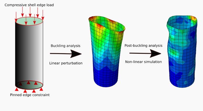
In an eigenvalue buckling problem we look for the loads for which the model stiffness matrix becomes singular, so that the problem
$$\K \v = 0$$has nontrivial solutions. $\K$ is the tangent stiffness matrix when the loads are applied, and the $\v$ are nontrivial displacement solutions.
Generals steps
Static general
A static stress analysis:
• is used when inertia effects can be neglected;
• can be linear or nonlinear; and
• ignores time-dependent material effects (creep, swelling, viscoelasticity) but takes rate-dependent plasticity and hysteretic behavior for hyperelastic materials into account.
where $\K$ is the stiffness matrix, $\u$ - is the vector of nodal displacements and $\F$ is the vector of external forces.
During a static step you assign a time period to the analysis. In some cases this time scale is quite real - for example, the response may be caused by temperatures varying with time based on a previous transient heat transfer run; or the material response may be rate dependent (rate-dependent plasticity), so that a natural time scale exists.
Static, Riks
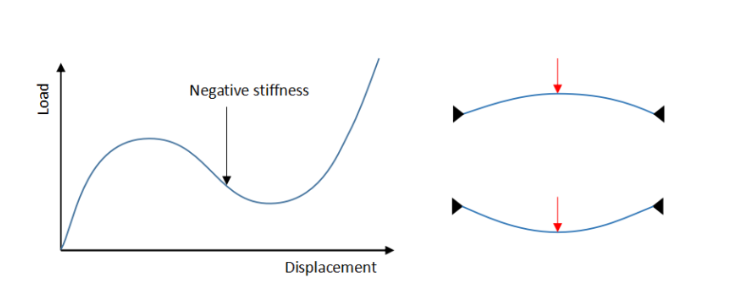
Geometrically nonlinear static problems sometimes involve buckling or collapse behavior, where the load-displacement response shows a negative stiffness, and the structure must release strain energy to remain in equilibrium. The modified Riks method allows you to find static equilibrium states during the unstable phase of the response.
Dynamic, explicit
An explicit, dynamic analysis is computationally efficient for the analysis of large models with relatively short dynamic response times and for the analysis of extremely discontinuous events or processes. This type of analysis allows for the definition of very general contact conditions and uses a consistent, large-deformation theory.
$$\dot{\u}_{(i+\frac12)} = \dot{\u}_{(i+\frac12)} + \cfrac{\Delta t_{(i+1)} + \Delta t_{(i)}}{2} \ddot{\u}_{(i)}$$ $$\u_{(i+1)} = \u_{(i)} + \Delta t_{(i+1)}\dot{\u}_{(i+\frac12)}$$where $\u$ is a degree of freedom (a displacement or rotation component) and the subscript $i$ refers to the increment number in an explicit dynamics step.
The key to the computational efficiency of the explicit procedure is the use of diagonal element mass matrices $\M$ because the accelerations $\ddot{\u}$ at the beginning of the increment are computed by
$$\ddot{\u}_{(i)} = \M^{-1} (\P_{(i)} - \I_{(i)})$$where $\P$ is the applied load vector, and $\I$ is the internal force vector.
Heat transfer
You can perform an uncoupled heat transfer analysis to model solid body heat conduction with general, temperature-dependent conductivity, , and general convection and radiation boundary conditions, including cavity radiation.
Steady-state analysis means that the internal energy term (the specific heat term) in the governing heat transfer equation is omitted. The problem then has no intrinsic physically meaningful time scale.
$$\rho c \dot{T} = - q_{i,i} + \rho r, \quad \rightarrow 0=- q_{i,i} + \rho r$$Transient analysis Time integration in transient problems is done with the backward Euler method. the relationship between the minimum usable time increment and the element size shuould be
$$\Delta t > \cfrac{\rho c}{6k} \Delta l^2$$where $\Delta t$ is the time increment, $\rho$ is the density, $c$ is the specific heat, $k$ is the thermal conductivity, and $\Delta l$ is a typical element dimension (such as the length of a side of an element).
Dynamic, implicit
General nonlinear dynamic analysis in Abaqus/Standard uses implicit time integration to calculate the transient dynamic or quasi-static response of a system. The procedure can be applied to a broad range of applications. Abaqus/Standard uses the Hilber-Hughes-Taylor time integration by default.
$$\M \ddot{\u} + \C \dot{\u} + \K \u = \F(t)$$ $$\u_{n+1} = \u_n +\Delta t \dot{\u}_n + \cfrac{(\Delta t)^2}{2} \left[ (1-2\beta)\ddot{\u}_n + 2\beta \ddot{\u}_{n+1}\right]$$ $$\dot{\u}_{n+1} = \dot{\u}_n + \Delta t \left[ (1-\gamma)\ddot{\u}_n + \gamma \ddot{\u}_{n+1} \right]$$Coupled temperature-displacement
This is a fully coupled, simultaneous heat transfer and stress procedure. A fully coupled temperature-displacement analysis must be configured when the stress analysis is influenced by the temperature distribution, and the temperature distribution is influenced by the stress solution
An exact implementation of Newton's method involves a nonsymmetric Jacobian matrix as is illustrated in the following matrix representation of the coupled equations
$$\begin{bmatrix} K_{uu} & K_{uT} \\ K_{Tu} & K_{TT} \\ \end{bmatrix} \begin{bmatrix} \Delta u \\ \Delta T \\ \end{bmatrix} = \begin{bmatrix} R_{u} \\ R_{T} \\ \end{bmatrix}$$where $\Delta u$ and $\Delta T$ are the respective corrections to the incremental displacement and temperature, $K_{ij}$ are submatrices of the fully coupled Jacobian matrix, and $R_u$ and $R_{T}$ are the mechanical and thermal residual vectors, respectively.
Coupled thermal-electrical
Joule heating arises when the energy dissipated by an electrical current flowing through a conductor is converted into thermal energy. Abaqus provides a fully coupled thermal-electrical procedure for analyzing this type of problem; the coupled thermal-electrical equations are solved simultaneously for both temperature and electrical potential at the nodes.
Coupled thermal-electrical-structural procedure
A fully coupled thermal-electrical-structural analysis is the union of
• a coupled thermal-displacement analysis
• a coupled thermal-electrical analysis.
Coupling between the temperature and electrical degrees of freedom arises from temperature-dependent electrical conductivity and internal heat generation (Joule heating), which is a function of the electrical current density.
Direct cyclic
A direct cyclic procedure is a quasi-static analysis that uses a combination of Fourier series and time integration of the nonlinear material behavior to obtain the stabilized cyclic response of the structure iteratively. The direct cyclic low-cycle fatigue capability provides a computationally effective technique for modeling progressive damage and failure.
Dynamics, Temp-disp, Explicit
Coupled temperature-displacement procedure using explicit integration.
Geostatic
A geostatic stress field procedure allows to verify that the initial geostatic stress field is in equilibrium with applied loads and boundary conditions. This type of procedure is usually the first step of a geotechnical analysis, followed by a coupled pore fluid diffusion/stress or static analysis procedure.
Mass diffusion
A mass diffusion analysis models the transient or steady-state diffusion of one material through another, such as the diffusion of hydrogen through a metal. The governing equations for mass diffusion are an extension of Fick's equations: they allow for nonuniform solubility of the diffusing substance in the base material and for mass diffusion driven by gradients of temperature and pressure
Soils
A coupled pore fluid diffusion/stress analysis allows to model single phase, partially or fully saturated fluid flow through porous media.
Visco
This procedure is used to analyze problems with time-dependent material response (creep, swelling, viscoelasticity). This type of analysis is valid when inertial effects can be neglected. It can be linear or nonlinear.
Abaqus increment and iteration
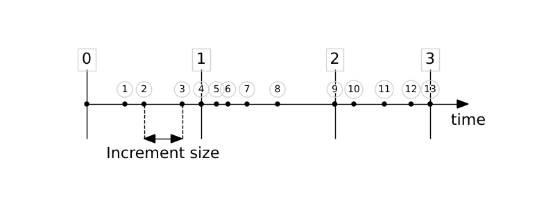
An increment is part of a step in Abaqus (Abaqus step). In nonlinear analyses, the total load applied in a step is broken into smaller increments so that the nonlinear solution path can be followed. Therefore, “Increment” is the part of the total load that is applied gradually.
This "Iteration" term is meaningful when we are using an implicit solver (Abaqus/Standard). There are no iterations in an ABAQUS/Explicit analysis.
In the case of an implicit solver, we seek the equilibrium after at every increment by checking the difference between externally applied force and internal reaction force. This difference is called residual.
The Abaqus/Standard solver uses the Newton method to solve nonlinear equilibrium equations. Many problems involve time-dependent responses, so the solution process typically consists of a series of increments along with trial-and-error iterations to reach equilibrium within each increment.
Sometimes, to achieve sufficient accuracy, these increments need to be small. The choice of increment size is often related to computational efficiency. If the number of increments is high, more trial-and-error iterations are required.
Abaqus Attempts
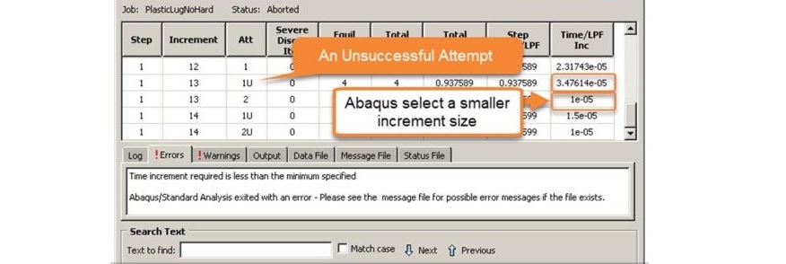
As explained before, Abaqus/Standard chooses the size of the increments automatically (except for the first increment). Every increment size selection in Abaqus is called an “attempt”. If Abaqus is unable to find a solution with the selected increment size after iterating several times, it makes a cutback in the increment size and begins a new attempt.
There are no attempts in an Abaqus/Explicit analysis!
Example: Metal forming
The analysis consists of four computational steps:
• the initial step, in which we define the positions of all parts,
• the second step involves applying pressure to the clamps,
• the third step is deformation, the movement of the punch,
• the fourth step is unloading.