Applied Continuum Mechanics with Abaqus

Introduction

In Abaqus, the term "Prescribed Conditions" generally refers to the boundary conditions that are imposed on a finite element model during an analysis. These conditions prescribe the values of certain degrees of freedom at specific nodes, essentially defining how the model interacts with its external environment.

The following types of external conditions can be prescribed in an Abaqus model:
• Initial conditions:
• Boundary conditions:
• Loads
• Predefined fields
• Load Case

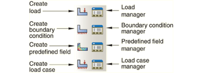
The Load Module toolbox in Abaqus provides a comprehensive platform for creating and editing loads, boundary conditions, predefined fields, and load cases.

Load module toolbox.

Initial conditions

In Abaqus, initial conditions refer to the state of the model at the beginning of a simulation. Initial conditions are specified for particular nodes or elements. If initial conditions are not specified, all initial conditions are zero. Abaqus allows users to specify various initial conditions depending on the type of analysis being performed. Here are some common examples:

• displacements

$$\u(\x,0) = \hat{\u}(\x)$$

• plastic strains

$$\ee^{pl}(\x,0) = \hat{\ee}^{pl}(\x)$$

• stresses

$$\ss(\x,0) = \hat{\ss}(\x)$$

• temperatures

$$T(\x,0) = \hat{T}(\x)$$

• velocities

$$\v(\x,0) = \hat{\v}(\x)$$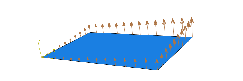

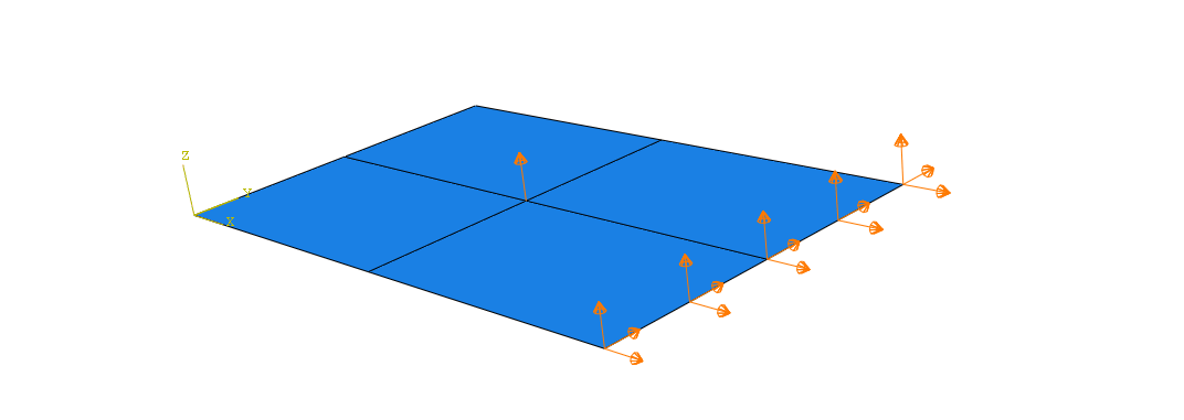
Initial values of velocity $v_3(x) = x+y$ generated in Abaqus/CAE.

Boundary conditions

Boundary conditions can be used to specify the values of all basic solution variables (displacements, rotations, temperatures) at nodes.

Almost every finite element analysis requires at least a set of boundary conditions.

Here are some common types of boundary conditions in Abaqus:
• displacement/rotation
• velocity/angular velocity
• acceleartion/angular acceleration
• temperature

Displacemnt boundary conditions.

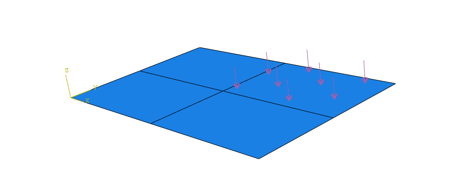
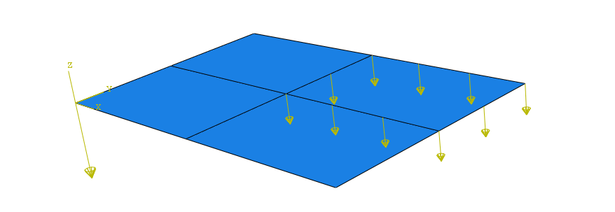
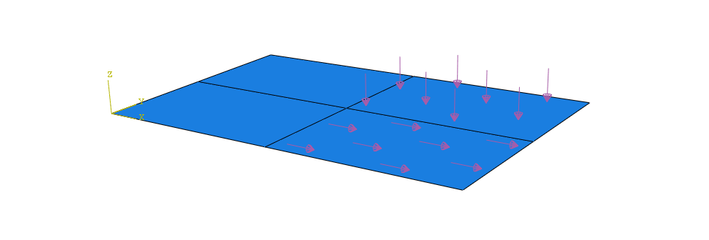
Loads

External loading can be applied in the following forms

• concentrated or distributed tractions.
• concentrated or distributed fluxes.

Concentrated loads:
• are applied to nodal degrees of freedom
• can be fixed in direction
• can rotate as the node rotates (referred to as follower forces), resulting in an additional, and possibly unsymmetric, contribution to the load stiffness

Distributed loads:
• can be prescribed on element faces, element bodies, or element edges
• can be prescribed over geometric surfaces or geometric edges;
• may be of follower type, which can rotate during a geometrically nonlinear analysis and result in an additional (often unsymmetric) contribution to the stiffness matrix.

Pressure load defined on the face.

Body Forces

Abaqus allows for definition of body forces. Body loads, such as gravity, are applied as element-based loads. The units of a body force are force per unit volume.

Body forces defined on the face and global gravity force .

Surface Traction and Pressure Loads

General or shear surface tractions and pressure loads can be applied in Abaqus as element-based or surface-based distributed loads. The units of these loads are force per unit area.

Pressure and traction defined on the face.

Thermal loads

Thermal loads can be applied in heat transfer analysis, in fully coupled temperature-displacement analysis. The following types of thermal loads are available:
• Concentrated heat flux prescribed at nodes.
• Distributed heat flux prescribed on element faces or surfaces.
• Body heat flux per unit volume.
• Boundary convection defined at nodes, on element faces, or on surfaces.
• Boundary radiation defined at nodes, on element faces, or on surfaces

Predefined fields

Abaqus allows for the definitions of the following types of predefined fields during an analysis:
• temperature
• field variables
• equivalent pressure stress
• mass flow rate

They can be defined:
• by entering the data directly
• by reading an Abaqus results file generated during a previous analysis (usually an
Abaqus/Standard heat transfer analysis)

Temperature can also be defined by reading an Abaqus output database file generated during a previous analysis. In Abaqus/Standard field variables can also be defined by reading an Abaqus output database file generated during a previous analysis.

Managing prescribed conditions

The prescribed condition managers are step-dependent managers, which means that they contain additional information concerning the history of each load, boundary condition, and predefined field in the model.

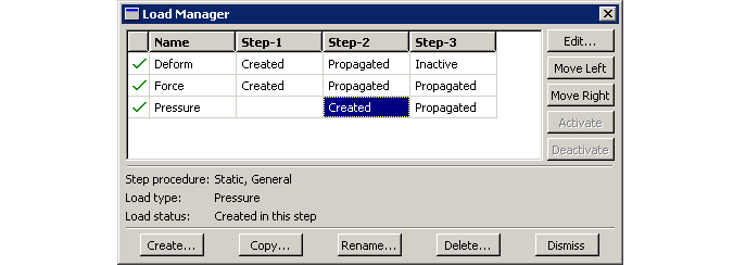
All prescribed conditions use the global coordinate system, with the exception of pressures, which are applied normal to the selected surfaces.The load and boundary condition allow to specify the coordinate system.

The Amplitude toolset

By default, the values of loads, boundary conditions, and predefined fields either change linearly with time throughout the step (ramp function) or they are applied immediately and remain constant throughout the step (step function).

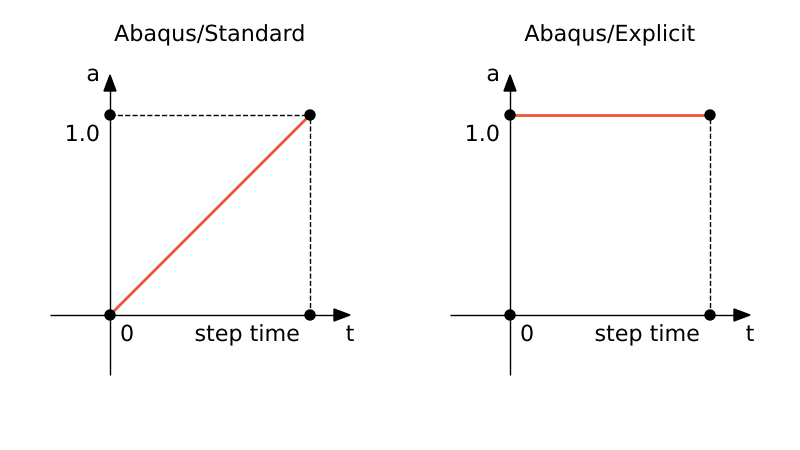
Default amplitudes for Abaqus solvers.

Amplitudes defined as functions of time can be given in terms of step time (default) or in terms of total time.

Types

Tabular - defines the amplitude curve as a table of values at convenient points on the time scale

Time	Relative load
0	0
1	1

Tabular amplitude definition.

An example of an amplitude function depending on time. Abaqus interpolates linearly between each time interval

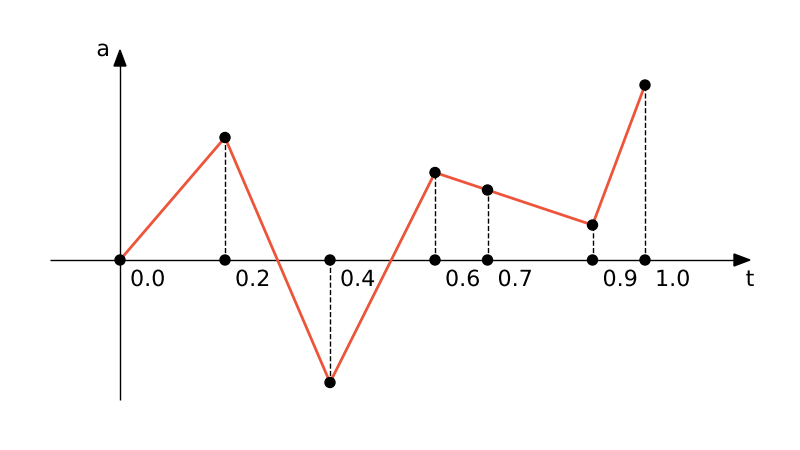
Equally spaced - gives a list of amplitude values at fixed time intervals beginning at a specified value of time.

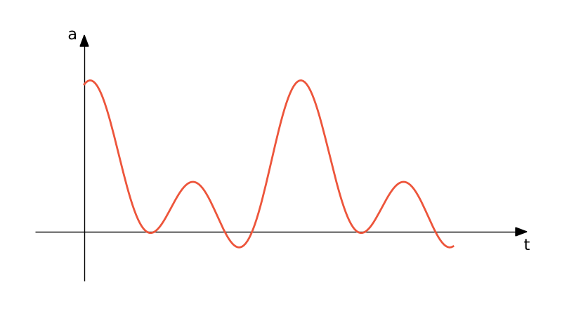
Periodic defines the amplitude, $a$, as a Fourier series

$$a = A_0 + \sum_{n=1}^N \left[A_n \cos \left(n \omega (t-t_0)\right)+ B_n\sin \left(n \omega (t-t_0)\right)\right], \quad \text{for} \quad t \geq t_0$$ $$a = A_0 \quad \text{for} \quad t < t_0$$

where $t_0$, $N$, $\omega$, $A_0$, $A_n$, and $B_n$ ,$n=1,2,...n$ are user-defined constants.

Example

Modulated

$$a = A_0 + A\sin \omega_1 (t-t_0) \sin \omega_2 (t-t_0) \quad \text{for} \quad t > t_0$$ $$a = A_0 \quad \text{for} \quad t < t_0$$

where $A_0$, $A$, $t_0$, $\omega_1$, and $\omega_2$ are user-defined constants.

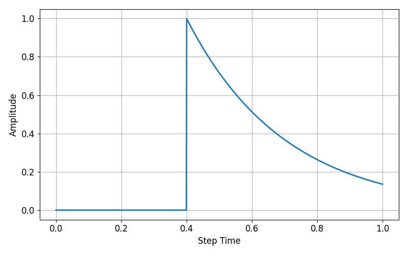
Decay

$$a = A_0 + A\exp\left( -(t-t_0)/t_d\right) \quad \text{for} \quad t \geq t 0$$ $$a = A_0 \quad \text{for} \quad t < t_0$$

where $A_0$, $A$, $t_0$ and $t_d$ are user-defined constants.

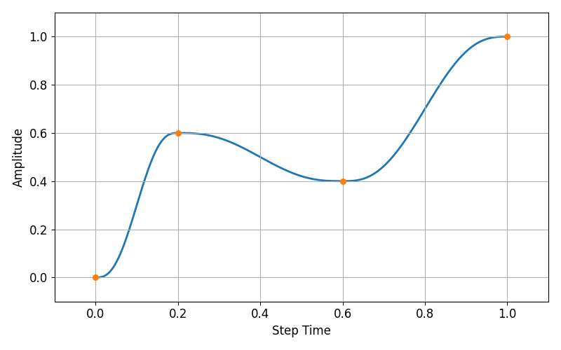
Smooth step
defines the amplitude, $a$, between two consecutive data points $(t_i, A_i)$ and $t_{i+1}, A_{i+1}$ as

$$a = A_i + (A_{i+1}-A_i)\xi^3(10-15\xi + 6 \xi^2) \quad \text{for} \quad t_i \leq t \leq t_{i+1}$$

where $\xi = (t-t_i)/(t_{i+1}-t_i) $

Analytical Field toolset

The Analytical Field toolset allows you to create and manage analytical fields. Analytical fields defined using mathematical expressions are called expression fields. Analytical fields indicate points in space using coordinates of the global coordinate system or of a local coordinate system.

Analytical Field toolset.

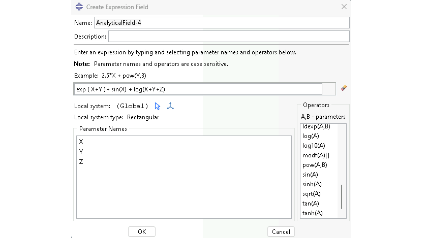
Example

f(X,Y) = sin(2X)

Pressure load distribution defined using analytical field.

The Discrete Field toolset

A discrete field is a spatially varying field where values are associated with a node or an element.

Discrete Field toolset.

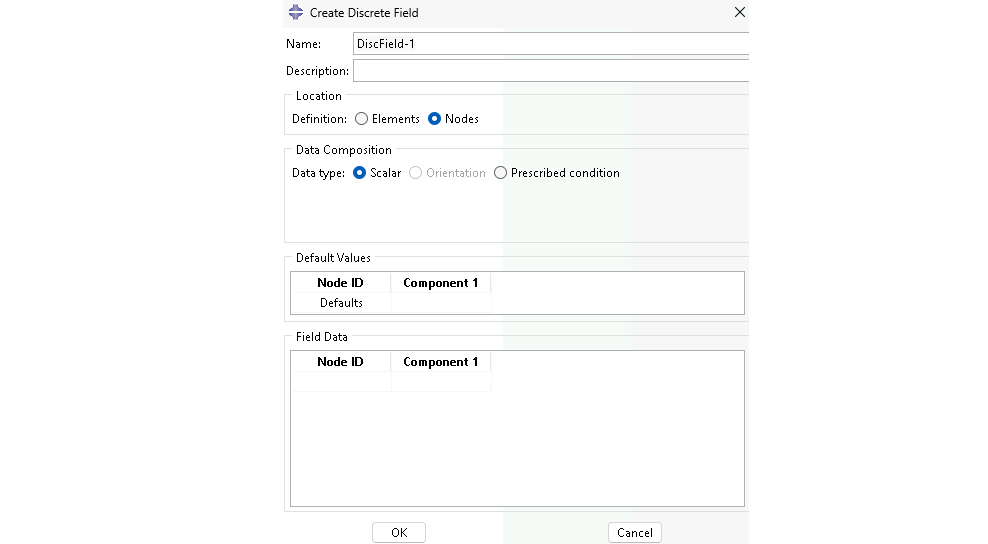
Example

Analysis of thermomechanical tension process for axisymmetric model

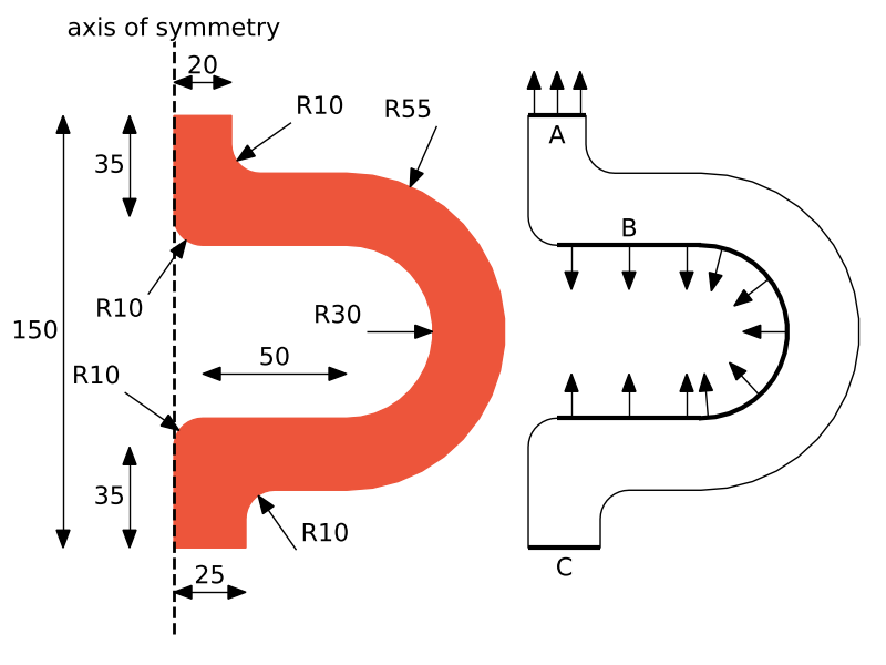
Material parameter	Value
Conductivity	0.5
Density	2000
Young's modulus	70 MPa
Poisson's ratio	0.3
Specific heat	2000

Assumptions:
• steady state analysis
• small strain theory
• linear isotropic elasticity

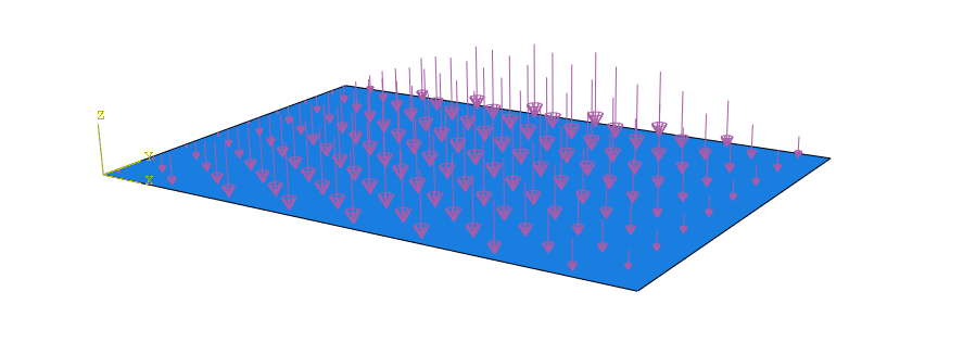
Boundary and initial conditions:
All - temperature $20^{\circ}$ at $t=0$,
A - pressure 1MPa, temperature $100^{\circ}$, distribution (analytical field) $20/(R+10)$,
B - heat flux,
C - temperature $20^{\circ}$

The developed example script can be downloaded at: