Constraints
In Abaqus, constraints play a crucial role in defining and controlling the behavior of a finite element model. They are essential for accurately representing real-world behavior in finite element simulations by controlling the relationships and interactions between different parts of a model. They provide a means to impose necessary conditions and constraints to obtain meaningful and accurate results during analysis.
Here are some common types of constraints used in Abaqus:
Tie
Two regions can be fused together by a tie constraint, even if the meshes created on the surfaces of the regions may be dissimilar.
Rigid body
The motion of regions of the assembly can be constrained to the motion of a reference point by a rigid body constraint. The relative positions of the regions that are part of the the rigid body remain constant throughout the analysis.
Display body
A display body constraint enables the selection of a part instance for display purposes only. The part instance does not need to be meshed, and it is excluded from the analysis. Nevertheless, when the results of the analysis are viewed, the selected part instance is displayed by the Visualization module. The part instance can be constrained to remain fixed in space, or it can be constrained to follow selected nodes.
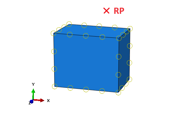
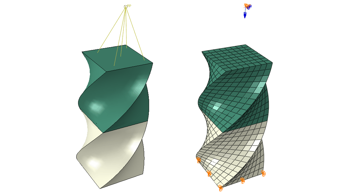
Coupling
The motion of a surface can be constrained to the motion of a single point by a coupling constraint.
MPC constraint
The motion of the slave nodes of a region can be constrained to the motion of a single point by an MPC (Multi-Point Constraint) constraint.
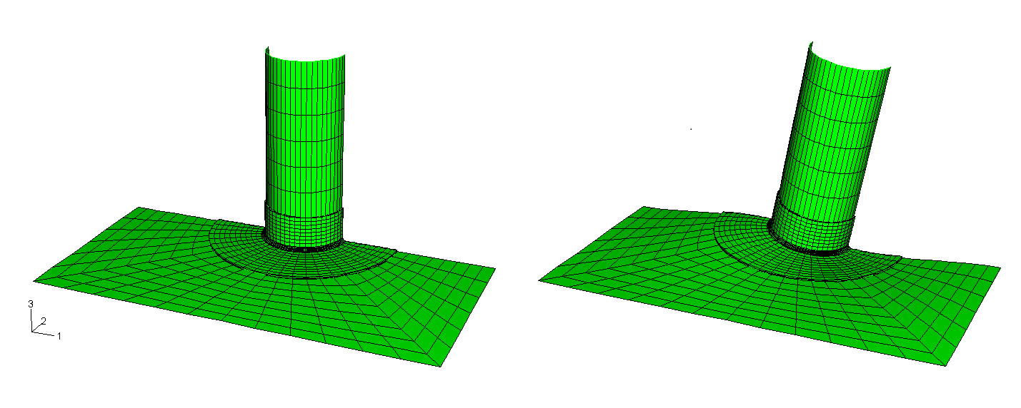
Shell-to-solid coupling
The motion of a shell edge can be coupled to the motion of an adjacent solid face by a shell-to-solid coupling constraint.
Equation
Linear, multi-point equation constraints known as equations allow the description of linear constraints between individual degrees of freedom.
Tie
A surface-based tie constraint can be used to make the translational and rotational motion as well as all other active degrees of freedom equal for a pair of surfaces. By default nodes are tied only where the surfaces are close to one another. One surface in the constraint is designated to be the slave surface; the other surface is the master surface.

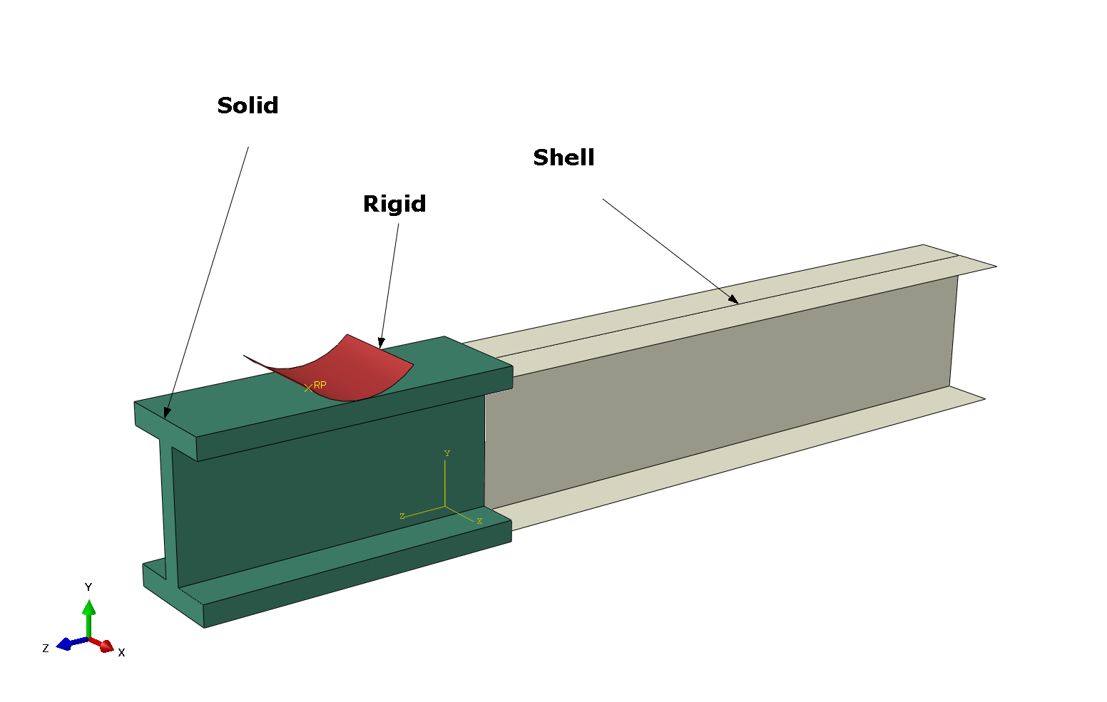
In Abaqus, tying two parts with incompatible meshes involves using the "Tie" constraint to connect surfaces or regions between the two parts. This is particularly useful when dealing with assemblies where the meshes on the connected parts do not match exactly.
Rigid body
A rigid body is a collection of nodes, elements, and/or surfaces whose motion is governed by the motion of a single node, called the rigid body reference node. The relative positions of the nodes and elements that are part of the rigid body remain constant throughout a simulation.
When a rigid body is not constrained fully, the mass and inertia properties of the rigid body are important to its dynamic response. In Abaqus/Explicit an error message will be issued if there is no mass (or rotary inertia) corresponding to an unconstrained degree of freedom.
Note
In Abaqus there are two ways to model rigid bodies - either by defining them as discrete or analytical rigid from the beginning (then the first type must be meshed with discrete rigid elements) or by defining them as deformable, meshing with regular elements and then applying the rigid body constraint. One of the advantages of the latter approach is that you can easily activate and deactivate the constraint switching between modeling the part as deformable and as rigid.
Rigid parts are associated with parts; rigid body constraints are associated with regions of the assembly. For example, if you define a part to be rigid, every instance of the part in the assembly is rigid.
Display body
The display body is used for display purposes only and does not take part in the analysis. It can be used to make the analysis more efficient while improving visualization of analysis results and is especially useful for mechanism or multibody dynamic analyses.
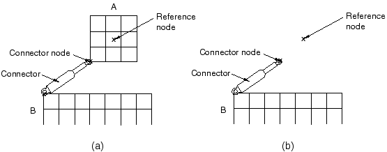
Part instance A is included in a display body definition. The figure shows the same model without the display body. This model will actually be involved in the analysis. The connector node and reference node form a rigid body that represents the analysis version of part instance A. Both these nodes are assembly-level nodes and are not included in the display body.
If the display body is not associated with any reference nodes, it will remain fixed in space during the analysis.
Coupling
The coupling constraint is useful when a group of coupling nodes are constrained to the rigid body motion of a single node. The coupling constraint can be effectively employed when applying loads or boundary conditions to a model.
Defining a coupling constraint requires the specification of the reference node (also called the constraint control point), the coupling nodes, and the constraint type. The coupling constraint associates the reference node with the coupling nodes.
MPC constraint
Multi-point constraints (MPCs) allow constraints to be imposed between different degrees of freedom of the model and can be quite general. Defining a coupling constraint requires the specification of the reference node (also called the constraint control point), the coupling nodes, and the constraint type. The coupling constraint associates the reference node with the coupling nodes
MPC types
Beam
is a rigid beam connection to constrain the displacement and rotation of each slave node to the displacement and rotation of the control point.
Tie
makes all active degrees of freedom equal at each slave node and the control point.
LINK
defines a pinned rigid link between each slave node and the control point.

The LINK connection constrains the position of node $b$, to a constant distance from node $a$.
Pin
defines a pinned joint between each slave node and the control point.

A pinned joint restricts translation in all directions and allows rotation
Shell-to-solid coupling
Surface-based shell-to-solid coupling:
• allows for a transition from shell element modeling to solid element modeling
• is most useful when local modeling should use a full three-dimensional analysis but other parts of the structure can be modeled as shells
• does not require any alignment between the solid and shell element meshes
Connectors
In Abaqus, connectors are elements used to model interactions between different parts of a structure. Connectors allow you to represent various types of physical connections, such as bolts, springs, or welds, between different regions or components in a finite element model.
To utilize connectors in Abaqus, you typically follow a process that involves creating an assembly-level wire feature, defining a connector section, and assigning this section to selected wires. The connector section specifies the mechanical properties and behavior of the connector.
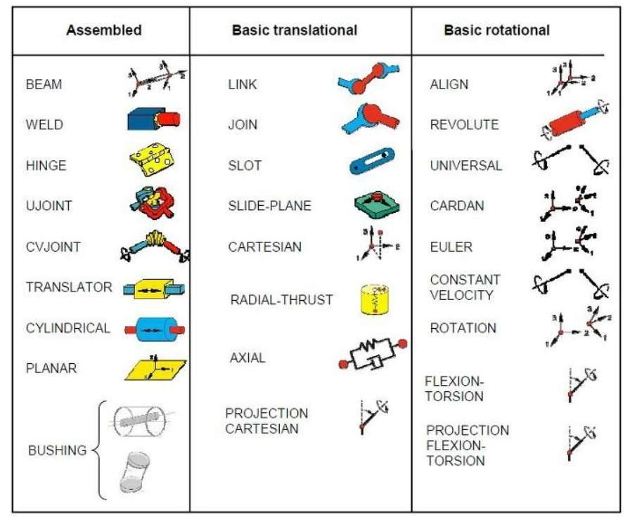
AXIAL
Provide a connection between two nodes that acts along the line connecting the nodes.
JOIN
Join the position of two nodes
ALIGN
Provide a connection between two nodes that aligns their local directions.
BEAM
Provide a rigid beam connection between two nodes. (JOIN + ALIGN)
REVOLUTE
Provide a revolute connection between two nodes.
HINGE
Join the position of two nodes, and provide a revolute connection between their rotational degrees of freedom. (JOIN + REVOLUTE)
Connector behaviors
In Abaqus, connector behaviors refer to the characteristics and responses of connectors, which are elements used to model interactions between different parts of a structure. Connector behaviors can be applied to connection types that have available components of relative motion.
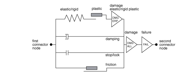
In a connector section, multiple connector behaviors can be defined, and the following connector behaviors can be specified:
Elasticity Define spring-like elastic behavior.
Damping Define dashpot-like damping behavior.
Friction Define Coulomb-like and hysteretic friction using predefined or user-defined friction models.
Plasticity Define plastic behavior.
Damage Define damage initiation and evolution behavior.
Stop Define limit values of the admissible range of positions.
Lock Specify a user-defined locking criterion.
Failure Define limit values for force, moment, or position.
Reference Length Define the translational or angular positions at which constitutive forces and moments are zero.
Example
Twisting of hyperelastic material with coupling constraint
The developed example script can be downloaded at: