Contact modeling
Abaqus provides more than one approach for defining contact. Abaqusincludes the following approaches for defining contact:
• general contact
• contact pairs
• contact elements
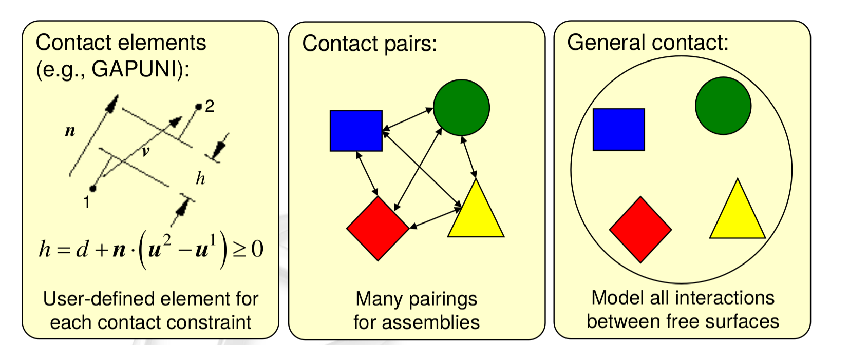
Each approach has somewhat unique advantages and limitations.
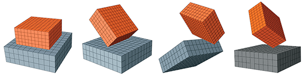
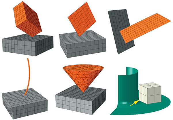
The general contact algorithm in Abaqus offers capabilities to model surface-to-surface contact, edge-to-surface contact, edge-to-edge contact, and vertex-to-surface contact. The surface-to-surface contact formulation is the primary formulation in that case with three-dimensional models.
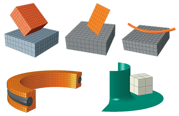
Edge-to-surface contact scenarios
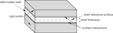
In Abaqus, the edge-to-surface contact is a type of contact interaction that allows modeling interactions between edges and surfaces. This type of contact is common in situations where you have a thin feature, such as a beam or a shell, interacting with a solid surface
Edge-to-edge contact scenarios
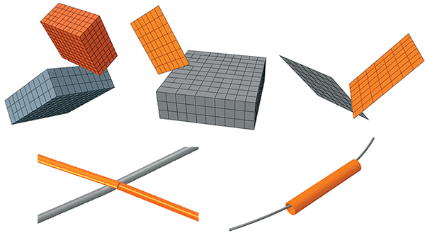
Vertex-to-surface contact scenarios
"Ingredients" of a Contact Model:
Contact surfaces
Surfaces over bodies that may experience contact
Contact interactions
Which surfaces interact with one another?
Surface property assignments
For example, contact thickness of a shell
Contact property models
Examples: pressure vs. overclosure relationship, friction coefficient, conduction coefficients, etc.
Contact formulation
For example, can a small-sliding formulation be used?
Surfaces
Surfaces can be defined at the beginning of a simulation or upon restart as part of the model definition. Abaqus has four classifications of contact surfaces:
• element-based deformable and rigid surfaces
• node-based deformable and rigid surfaces
• analytical rigid surfaces
• Eulerian material surfaces for Abaqus/Explicit
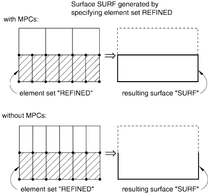
Element-based deformable and rigid surfaces
For element-based surfaces Abaqus uses a faceted geometry defined by the finite element mesh as the surface definition. The surface in a coarse finite element model may not be a very good approximation for contact modeling if the physical surface is curved. Therefore, sufficient mesh refinement must be used to ensure that the faceted surface is a reasonable approximation of the curved physical surface
Node-based deformable and rigid surfaces
You create a node-based surface by specifying the nodes or node sets that form the surface.
Analytical rigid surface
Analytical rigid surfaces are geometric surfaces with profiles that can be described with straight and curved line segments. These profiles can be swept along a generator vector or rotated about an axis to form a three-dimensional surface. An analytical rigid surface is associated with a rigid body reference node, whose motion governs the motion of the surface.
Eulerian surface
An Eulerian surface represents the exterior surface of a particular Eulerian material instance in an Abaqus/Explicit analysis. Since Eulerian materials flow through the Eulerian mesh, their surfaces cannot be defined by a simple list of element faces. Instead, these surfaces often lie within Eulerian elements and must be computed in each time increment using element volume fraction data.
Contact interactions
Contact interactions for contact pairs and general contact are defined by specifying surface pairings and self-contact surfaces. General contact interactions typically are defined by specifying self-contact for the default surface, which allows an easy, yet powerful, definition of contact. (Self-contact for a surface that spans multiple bodies implies self-contact for each body as well as contact between the bodies.)
Surface properties
Nondefault surface properties (such as thickness and, in some cases, offset) can be defined for particular surfaces in a contact model.
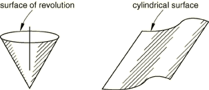
Smoothing contact surface
Three geometry correction methods can be employed:
• The circumferential smoothing method is applicable to surfaces approximating a portion of a circle in two dimensions or a portion of a surface of revolution in three dimensions.
• The spherical smoothing method is applicable to surfaces approximating a portion of a sphere in three dimensions.
• The toroidal smoothing method is applicable to surfaces approximating a portion of a torus in three dimensions (i.e., a circular arc revolved about an axis).
Contact properties
By default, the surfaces have constraints only in the normal direction to resist penetration. The other mechanical contact interaction models available depend on the contact algorithm. Some of the available models are:
• pressure-overclosure
• friction
Pressure-overclosure relationships
In Abaqus the following contact pressure-overclosure relationships can be used to define the contact model:
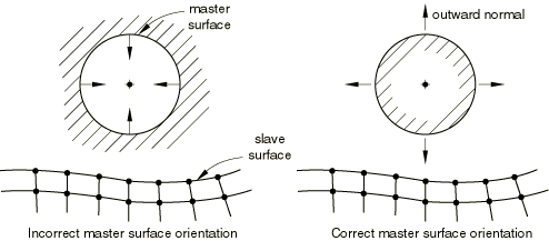
• the “hard” contact relationship minimizes the penetration of the slave surface into the master surface at the constraint locations and does not allow the transfer of tensile stress across the interface;
• a “softened” contact relationship in which the contact pressure is a linear function of the clearance between the surfaces;
• a “softened” contact relationship in which the contact pressure is an exponential function of the clearance between the surfaces
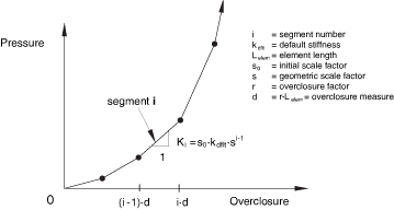
• a “softened” contact relationship in which a tabular pressure-overclosure curve is constructed by progressively scaling the default penalty stiffness
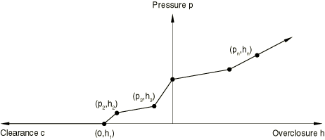
• a “softened” contact relationship in which the contact pressure is a piecewise linear (tabular) function of the clearance between the surfaces
• a relationship in which there is no separation of the surfaces once they contact.
“hard” contact relationship
When surfaces are in contact, any contact pressure can be transmitted between them. The surfaces separate if the contact pressure reduces to zero. Separated surfaces come into contact when the clearance between them reduces to zero.

“Softened” contact defined as a linear function
In a linear pressure-overclosure relationship the surfaces transmit contact pressure when the overclosure between them, measured in the contact (normal) direction, is greater than zero. The linear pressure-overclosure relationship is identical to a tabular relationship with two data points, where the first point is located at the origin.
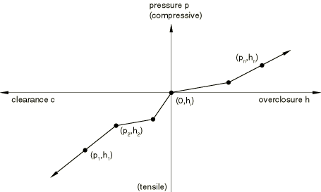
“Softened” contact defined in tabular form.
To define a piecewise-linear pressure-overclosure relationship in tabular form, as shown in Figure 37.1.2–2, you specify data pairs (, ) of pressure versus overclosure (where overclosure corresponds to negative clearance). You must specify the data as an increasing function of pressure and overclosure.
“Softened” contact defined as a geometric scaling of the default contact stiffness
An alternative piecewise linear tabular pressure-overclosure relationship can be constructed by geometrically scaling the default contact stiffness. This model provides a simple interface to increase the default contact stiffness when a critical penetration is exceeded.
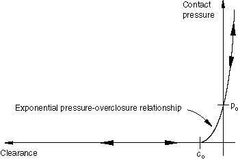
“Softened” contact defined with an exponential law
In an exponential (soft) contact pressure-overclosure relationship the surfaces begin to transmit contact pressure once the clearance between them, measured in the contact (normal) direction, reduces to . The contact pressure transmitted between the surfaces then increases exponentially as the clearance continues to diminish.
Using the no separation relationship
You can indicate that Abaqus should use the contact pressure-overclosure relationship that prevents surfaces from separating once they have come into contact. In Abaqus/Explicit this relationship can be specified for general contact but only for pure master-slave contact pairs, and it cannot be used with adaptive meshing.
Frictional behavior
When surfaces are in contact they usually transmit shear as well as normal forces across their interface. There is generally a relationship between these two force components. The relationship, known as the friction between the contacting bodies, is usually expressed in terms of the stresses at the interface of the bodies. The friction models available in Abaqus:
• include the classical isotropic Coulomb friction model
• in its general form allows the friction coefficient to be defined in terms of slip rate, contact pressure, average surface temperature at the contact point
• provides the option for you to define a static and a kinetic friction coefficient with a smooth transition zone defined by an exponential curve;
• allow the introduction of a shear stress limit, which is the maximum value of shear stress that can be carried by the interface before the surfaces begin to slide;
• include an anisotropic extension of the basic Coulomb friction model
Using the basic Coulomb friction model
The basic concept of the Coulomb friction model is to relate the maximum allowable frictional (shear) stress across an interface to the contact pressure between the contacting bodies.
The Coulomb friction model defines tcritical shear stress, $\tau_{crit}$, at which sliding of the surfaces starts as a fraction of the contact pressure, $p$, between the surfaces
$$\tau_{crit} = \mu p$$The fraction, $\mu$ , is known as the coefficient of friction.
Abaqus combines the two shear stress components into an “equivalent shear stress,” $\bar{\tau}$, for the stick/slip calculations, where .
$$\bar{\tau} = \sqrt{\tau_1^2 + \tau^2_2}$$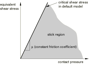
Contact Formulations
Abaqus provides several contact fomulations. Each formulation is based on a choice of
• a contact discretization
• a tracking approach
• ssignment of “master” and “slave” roles to the contact surfaces.
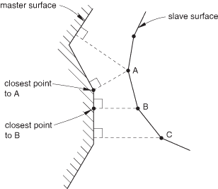
Discretization of contact pair surfaces
With traditional node-to-surface discretization the contact conditions are established such that each “slave” node on one side of a contact interface effectively interacts with a point of projection on the “master” surface on the opposite side of the contact interface.
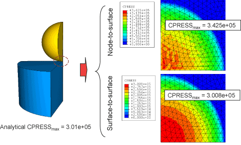
Surface-to-surface contact discretization
In general, surface-to-surface discretization provides more accurate stress and pressure results than node-to-surface discretization if the surface geometry is reasonably well represented by the contact surfaces
Contact tracking approaches
In Abaqus/Standard there are two tracking approaches to account for the relative motion of two interacting surfaces in mechanical contact simulations.
• The finite-sliding tracking approach
Finite-sliding contact is the most general tracking approach and allows for arbitrary relative separation, sliding, and rotation of the contacting surfaces.
• The small-sliding tracking approach
Small-sliding contact assumes that there will be relatively little sliding of one surface along the other and is based on linearized approximations of the main surface per constraint.
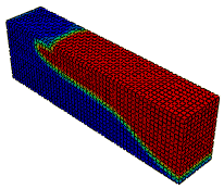
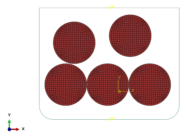
Example
Contact modeling for the disk crushing process
The developed example script can be downloaded at: