Abaqus Meshing
Meshing is a fundamental aspect of Finite Element Analysis (FEA) in which large, complex geometries are discretized into a set of simple, interconnected elements.
In Abaqus/CAE the Mesh module allows you to generate meshes on parts and assemblies. The process of assigning mesh attributes to the model is feature based. As a result you can modify the parameters that define a part or an assembly, and the mesh attributes that you specified within the Mesh module are regenerated automatically.
The Mesh module provides the following features:
• Tools for prescribing mesh density at local and global levels.
• Model coloring that indicates the meshing technique assigned to each region in the model.
• A variety of mesh controls, such as:
• Element shape
• Meshing technique
• Meshing algorithm
• Adaptive remeshing rule
• A tool for verifying mesh quality.
• Tools for refining the mesh and for improving the mesh quality.
The meshing process
To create an acceptable mesh, you use the following process:
• Assign mesh attributes and set mesh controls
• Generate the mesh
• Refine the mesh
• Optimize the mesh
• Verify the mesh
Mesh attributes and controls
Mesh seeds
The target mesh density in a region is specified by placing markers, known as seeds, along its edges. Both the mesh density along the boundary of the region and the mesh density in the interior of the region are influenced by the seeds along the edges of the region.
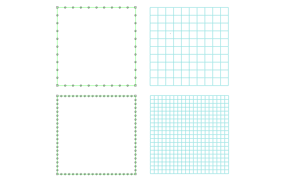
Abaqus/CAE generates meshes that match your seeds as closely as possible. Abaqus/CAE can use the following methods to control the distribution of the seeds:
• position the seeds uniformly along all the edges of a part or part instance
• position the seeds uniformly along an edge
• position the seeds with a bias such that the mesh density increases toward one end of the edge
• position the seeds with a bias such that the mesh density increases from each end toward the center of the edge
• position the seeds with a bias such that the mesh density increases from the center toward each end of the edge
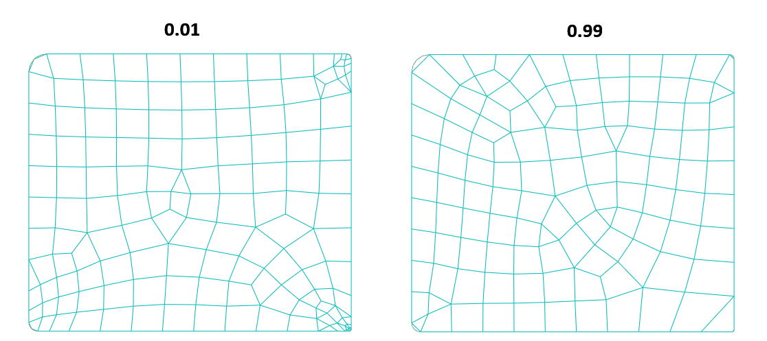
Applying curvature control to seeding
To avoid the problem of inadequate seeding around small curved features, Abaqus/CAE applies curvature control when it seeds a part.
The curve control is set by a specified
• deviation factor
• minimum size factor.
The deviation factor is a measure of how much the element edges deviate from the original geometry

The minimum size factor prevents Abaqus/CAE from creating very fine meshes in areas of high curvature that are of no interest in modeling, for example: fillets with a very small radius.
This factor's minimum size is determined as a fraction of the global seed size
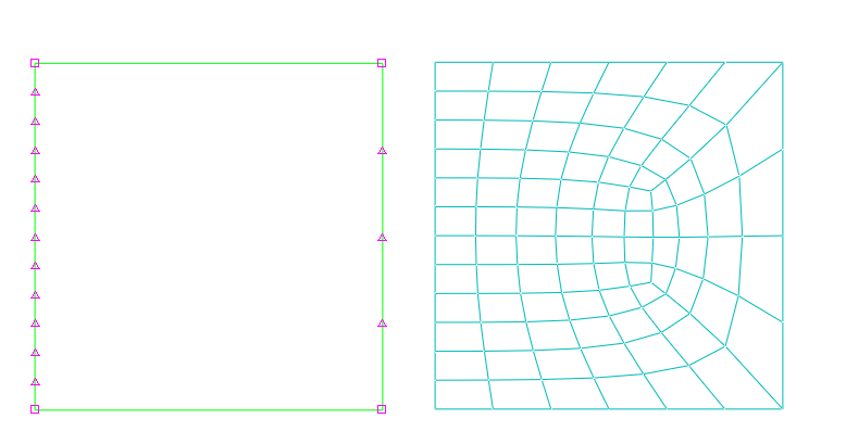
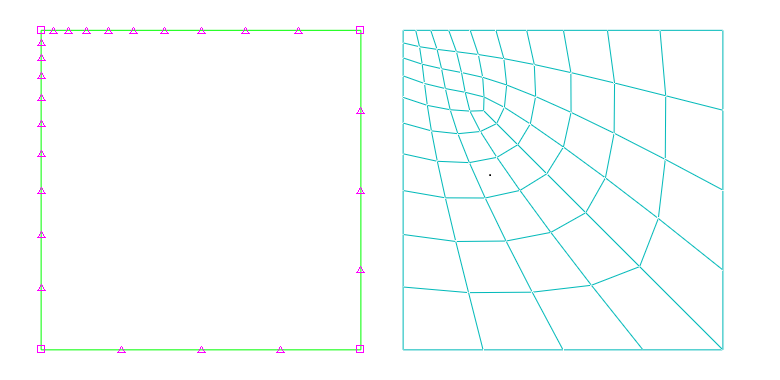
Constraining seeds
By default, mesh seeds prescribe only a target mesh density. Abaqus/CAE generally matches the mesh seeds exactly. However, in some cases Abaqus/CAE may alter the element distribution so that it can successfully generate the mesh.
Three states can be assigned to a group of seeds along an edge
Unconstrained This is the default setting. The number of elements along an edge can either increase or decrease so that the mesh can become denser or coarser than is specified by the seeds. Unconstrained seeds appear as open circles.
Partially constrained The number of elements along an edge may be increased during mesh generation but cannot be decreased. This constraint allows the mesh to become denser than is specified by the seeds but no coarser. Partially constrained seeds appear as upward-pointing triangles.
Fully constrained The number of elements specified by constrained seeds along an edge cannot be altered by the mesh generation process. Fully constrained seeds appear as squares.
Abaqus/CAE always creates a fully constrained seed at each geometric vertex of a region to indicate that a finite element node will be positioned at each vertex.
Mesh generation
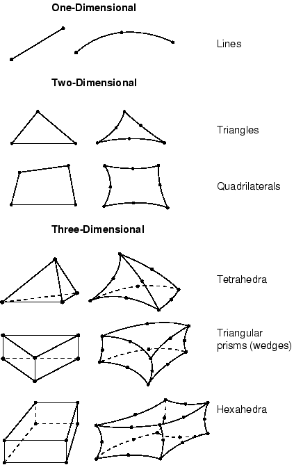
Abaqus/CAE can use a variety of meshing techniques to mesh models of different topologies.
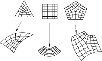
• Structured meshing
The structured meshing technique generates structured meshes using simple predefined mesh topologies. Abaqus/CAE transforms the mesh of a regularly shaped region, such as a square or a cube, onto the geometry of the region you want to mesh.
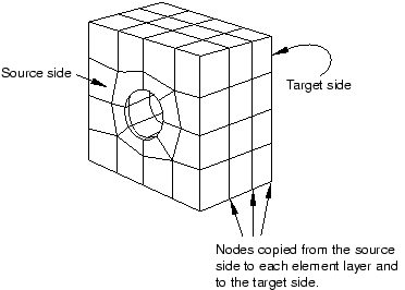
• Swept meshing
Abaqus/CAE creates swept meshes by internally generating the mesh on an edge or face and then sweeping that mesh along a sweep path. The result can be either a two-dimensional mesh created from an edge or a three-dimensional mesh created from a face.
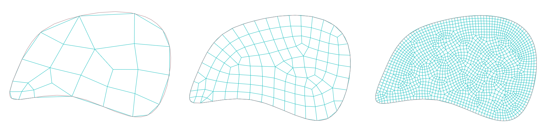
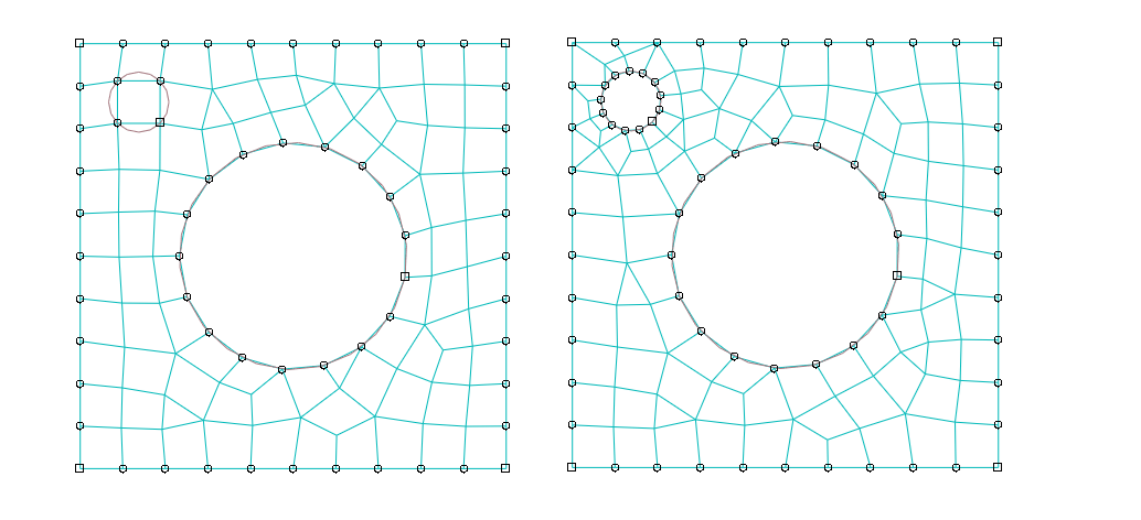
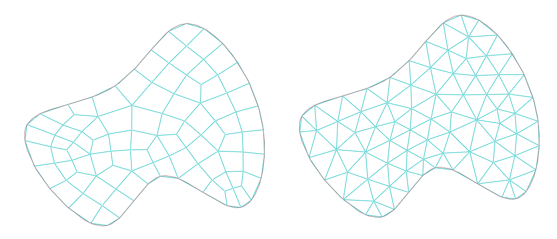
• Free meshing
The free meshing technique is the most flexible top-down meshing technique. It uses no preestablished mesh patterns and can be applied to almost any model shape. However, free meshing provides you with the least control over the mesh since there is no way to predict the mesh pattern. Figure 17–5 shows an example of a free mesh
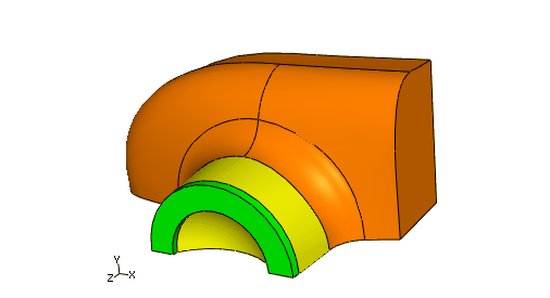
Mesh technique color coding
Abaqus/CAE uses different colors to indicate which meshing technique, if any, is currently assigned to a region.
| color | meshing technique |
|---|---|
| green | structured |
| yellow | sweep |
| pink | free |
| orange | unmeshable |
Mesh refinement
The Mesh module provides a set of tools that allow you to refine a mesh.
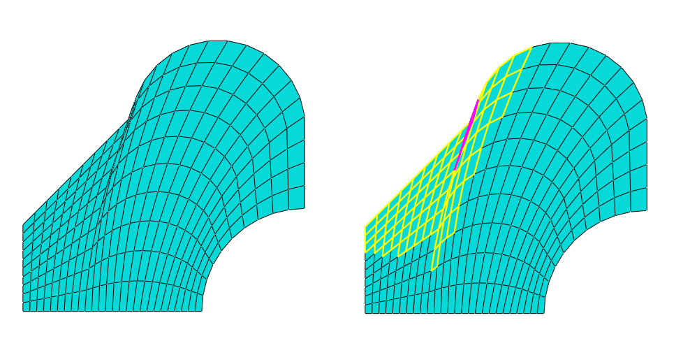
Partition toolset is used to divide geometric regions into smaller regions. The resulting partitions introduce new edges that you can seed therefore, you can combine partitioning and seeding to gain additional control over the mesh generation process.
The Virtual Topology In some cases the geometry contains details such as very small faces and edges. The Virtual Topology toolset allows to remove these small details by combining a small face with an adjacent face or by combining a small edge with an adjacent edge.
Edit Mesh toolset allows to make minor adjustments to your mesh
Mesh optimization
Remeshing rules can be assigned to regions of your model. Remeshing rules enable successive refinement of your mesh based on solution results.
The remeshing rule allows for specification:
• The region where you want the mesh refined.
• The solution quality criteria (for example error indicators in the Mises stress) that mesh refinement is based on.
• The analysis step or steps that refinement is based on.
• Minimum and maximum element size constraints.
• A sizing algorithm and parameters appropriate to your simulation.
Mesh verification
The Mesh module provides a set of tools that allow to verify a mesh and to obtain mesh statistics and mesh information. You can use the Shape metrics to highlight elements of a selected shape that do not meet one of the following selection criteria
• Shape factor
Abaqus/CAE highlights elements with a normalized shape factor smaller than a specified value. sThe shape factor ranges from 0 to 1, with 1 indicating the optimal element shape and 0 indicating a degenerate element.
For triangular elements the normalized shape factor is defined as
$$shape\,factor = \cfrac{element \, area}{optimal \, element \,area}$$For tetrahedral elements the normalized shape factor is defined as
$$shape \,factor = \cfrac{element \, volume}{optimal \, element \, volume}$$• Small face corner angle
Abaqus/CAE highlights elements containing faces where two edges meet at an angle smaller than a specified angle
• Large face corner angle
Abaqus/CAE highlights elements containing faces where two edges meet at an angle larger than a specified angle.
• Aspect ratio
Abaqus/CAE highlights elements with an aspect ratio larger than a specified value. The aspect ratio is the ratio between the longest and shortest edge of an element.
Meshing independent and dependent part instances
• Independent
You cannot mesh a part that you have used to create an independent instance.
• Dependent
Abaqus/CAE applies the same mesh to each dependent instance in the assembly. Dependent instances are convenient when you have a linear or radial pattern of part instances. You can mesh the original part, and Abaqus/CAE applies the same mesh to each instance of the part in the pattern.
Mesh transition
A mesh transition is an area where a mesh transitions from coarse (large elements) to fine (small elements)
Abaqus/CAE provides mesh transition controls for the following types of meshes:
• A two-dimensional, quadrilateral-only mesh that is created using the structured meshing technique or the free meshing technique with the medial axis algorithm.
A three-dimensional, hexahedral-only mesh that is created by sweeping a two-dimensional mesh.
Assigning Abaqus element types
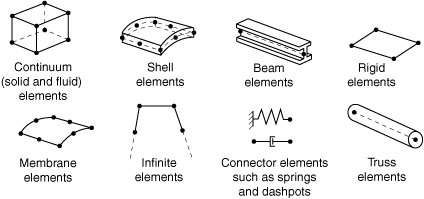
The Mesh module can generate meshes containing different element shapes.
Element library
Abaqus has an extensive element library to provide a powerful set of tools for solving many different problems.
Abaqus has an extensive element library to provide a powerful set of tools for solving many different problems.
Five aspects of an element characterize its behavior:
• Family
• Degrees of freedom (directly related to the element family)
• Number of nodes
• Formulation
• Integration
Family
Figure 27.1.1–1 shows the element families that are used most commonly in a stress analysis; in addition, continuum (fluid) elements are used in a fluid analysis. One of the major distinctions between different element families is the geometry type that each family assumes.
The first letter or letters of an element's name indicate to which family the element belongs. For example, S4R is a shell element, CINPE4 is an infinite element, and C3D8I is a continuum element.
Degrees of freedom
The degrees of freedom (dof) are the fundamental variables calculated during the analysis. For a stress/displacement simulation the degrees of freedom are the translations at each node. Some element families, such as the beam and shell families, have rotational degrees of freedom as well. For a heat transfer simulation the degrees of freedom are the temperatures at each node; a heat transfer analysis, therefore, requires the use of different elements than a stress analysis, since the degrees of freedom are not the same.
The following numbering convention is used for the degrees of freedom in Abaqus:
• 1 Translation in direction 1
• 2 Translation in direction 2
• 3 Translation in direction 3
• 4 Rotation about the 1-axis
• 5 Rotation about the 2-axis
• 6 Rotation about the 3-axis
• 7 Warping in open-section beam elements
• 8 Acoustic pressure, pore pressure, or hydrostatic fluid pressure
• 9 Electric potential
• 10 Connector material flow (units of length)
• 11 Temperature (or normalized concentration in mass diffusion analysis) for continuum elements or temperature at the first point through the thickness of beams and shells
• 12+ Temperature at other points through the thickness of beams and shells
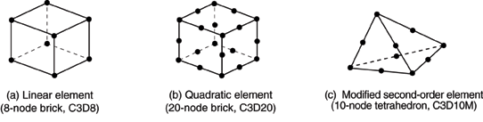
Number of nodes and order of interpolation
Displacements or other degrees of freedom are calculated at the nodes of the element. At any other point in the element, the displacements are obtained by interpolating from the nodal displacements. Usually the interpolation order is determined by the number of nodes used in the element.
Elements that have nodes only at their corners use linear interpolation in each direction and are often called linear elements or first-order elements.
In Abaqus/Standard elements with midside nodes use quadratic interpolation and are often called quadratic elements or second-order elements.
Modified triangular or tetrahedral elements with midside nodes, such as the 10-node tetrahedron shown in Figure 27.1.1–2(c), use a modified second-order interpolation and are often called modified or modified second-order elements.
Formulation
In the absence of adaptive meshing all of the stress/displacement elements in Abaqus are based on the Lagrangian or material description of behavior: the material associated with an element remains associated with the element throughout the analysis, and material cannot flow across element boundaries. In the alternative Eulerian or spatial description, elements are fixed in space as the material flows through them. Eulerian methods are used commonly in fluid mechanics simulations.
Integration
Abaqus uses numerical techniques to integrate various quantities over the volume of each element. Using Gaussian quadrature for most elements, Abaqus evaluates the material response at each integration point in each element. Some elements in Abaqus can use full or reduced integration.
Abaqus uses the letter “R” at the end of the element name to distinguish reduced-integration elements.
Element naming convention
The naming conventions for solid elements depend on the element dimensionality.
For example:
C3D20 is three dimensional continuum stress/displacment, 20-node element
CAX4R is an axisymmetric continuum stress/displacement, 4-node, reduced-integration element
CPS8RE is an 8-node, reduced-integration, plane stress piezoelectric element.
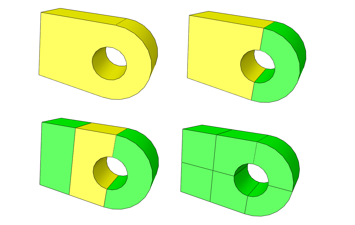
Example
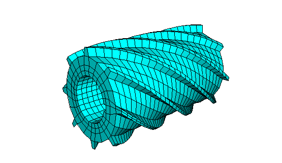
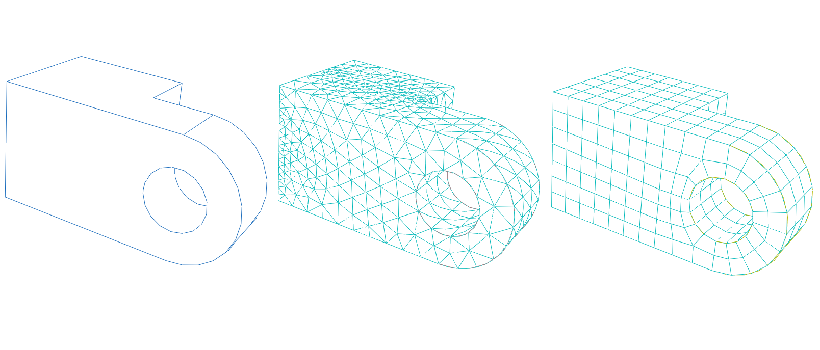
Generation of a three-dimensional mesh for geometry as shown in the picture below.
The developed example script can be downloaded at: