The review of material models in Abaqus
Abaqus has an extensive material library which can be used to model many engineering materials, including metals, rubbers, concrete, damage and failure, fabrics, and hydrodynamics. Abaqus also provides the facilities to create and use a user-defined material model for the purpose of finite element simulation.
Linear elasticity
A linear elastic material model:
• is valid for small elastis strains
• can be isotropic, orthotroic, or fully anisotropic
• can have properties that depend on temperature and/or other field variables
The total stress is defined from the total elastic strain as
$$\ss = \D \cdot \ee$$where $\ss$ is the total stress (“true,” or Cauchy stress in finite-strain problems), $\D$ is the fourth-order elasticity tensor, and $\ee$ is the total elastic strain (log strain in finite-strain problems).
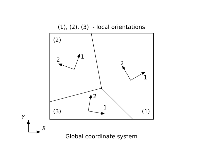
Depending on the number of symmetry planes for the elastic properties, a material can be classified as either isotropic (an infinite number of symmetry planes passing through every point) or anisotropic (no symmetry planes). If the material is anisotropic, a local orientation must be used to define the direction of anisotropy.
• Isotropic, two material constants, Young's modulus $E$ and Poisson's ratio $\nu$
$$\begin{bmatrix}\sigma _{11}\\\sigma _{22}\\\sigma _{33}\\\sigma _{12}\\\sigma _{13}\\\sigma _{23}\end{bmatrix}\,=\,\cfrac {E}{(1+\nu )(1-2\nu )}\begin{bmatrix}1-\nu &\nu &\nu &0&0&0\\ &1-\nu &\nu &0&0&0\\ & &1-\nu &0&0&0\\&&&{\frac {1-2\nu }{2}}&0&0\\&sym& & &{\frac {1-2\nu }{2}}&0\\&&&&&{\frac {1-2\nu }{2}}\end{bmatrix}\begin{bmatrix}\varepsilon _{11}\\\varepsilon _{22}\\\varepsilon _{33}\\\gamma _{12}\\\gamma_{13}\\\gamma _{23}\end{bmatrix}$$• Orthotropic, requires dircet specification of all nonzero terms
$$\begin{bmatrix}\sigma _{11}\\\sigma _{22}\\\sigma _{33}\\\sigma _{12}\\\sigma _{13}\\\sigma_{23}\end{bmatrix}=\begin{bmatrix}D_{1111}&D_{1122}&D_{1133}&0&0&0\\ &D_{2222}&D_{2233}&0&0&0\\&&D_{3333}&0&0&0\\&&&D_{1212}&0&0\\ &sym&&&D_{1313}&0\\&&&&&D_{2323}\end{bmatrix}\begin{bmatrix}\varepsilon _{11}\\\varepsilon _{22}\\\varepsilon _{32}\\\gamma _{12}\\\gamma _{13}\\\gamma _{23}\end{bmatrix}$$or we can use the engineering constants
$$E_1, \, E_2,\, E_3,\, \nu_{12},\, \nu_{13},\, \nu_{23},\, G_{12},\, G_{13},\, G_{23}$$• Anisotropic, requires dircet specification of all nonzero terms
$$\begin{bmatrix}\sigma _{11}\\\sigma _{22}\\\sigma _{33}\\\sigma _{12}\\\sigma _{13}\\\sigma_{23}\end{bmatrix}=\begin{bmatrix}D_{1111}&D_{1122}&D_{1133}&D_{1112}&D_{1113}&D_{1123}\\&D_{2222}&D_{2233}&D_{2212}&D_{2213}&D_{2223}\\&&D_{3333}&D_{3312}&D_{3313}&D_{3323}\\&&&D_{1212}&D_{1213}&D_{1223}\\&sym&&&D_{1313}&D_{1323}\\&&&&&D_{2323}\end{bmatrix}\begin{bmatrix}\varepsilon _{11}\\\varepsilon _{22}\\\varepsilon_{33}\\\gamma_{12}\\\gamma_{13}\\\gamma_{23}\end{bmatrix}$$Plane stress orthotropic failure measures
The orthotropic plane stress failure measures:
• are indication of material failure (normally used for fiber-reinforce composite materials)
• five different failure theories are provided: four stress based theories and on strain based theory
The input data for the stress-based failure theories are tensile and compressive stress limits, $X_t$ and $X_c$, in the 1-direction; tensile and compressive stress limits, $Y_t$ and $Y_c$ in the 2-direction; and shear strength (maximum shear stress), $S$, in the X–Y plane.
Maximum stress
If $\sigma_{11}>0, X=X_c$ otherwise $X=X_c$. If $\sigma_{22}>0, \, Y=0$ otherwise $Y=Y_c$. The maximum stress failure criterion requires that
$$I_f = \max\left( \cfrac{\sigma_{11}}{X}, \cfrac{\sigma_{22}}{Y}, \left|\cfrac{\sigma_{12}}{S}\right|\right)> 1.0$$Tsai-Hill
If $\sigma_{11}>0, X=X_c$ otherwise $X=X_c$. If $\sigma_{22}>0, \, Y=0$ otherwise $Y=Y_c$. The maximum stress failure criterion requires that
$$I_f = \cfrac{\sigma_{11}^2}{X^2} - \cfrac{\sigma_{11}\sigma_{22}}{X^2} + \cfrac{\sigma_{22}^2}{Y^2} + \cfrac{\sigma_{12}^2}{S^2}<1.0$$Tsai-Wu
$$I_F = F_1\sigma_{11} + F_2\sigma_{22} F_{11}\sigma_{11}^2+F_{22}\sigma_{22}^2 + F_{66}\sigma_{12}^2 + 2F_{12}\sigma_{11}\sigma_{22} < 1.0$$The Tsai-Wu coefficients are defined as follows
$$F_1=\cfrac{1}{X_t} + \cfrac{1}{X_c}, \quad F_2=\cfrac{1}{Y_t} + \cfrac{1}{Y_c}, \quad F_{11}=-\cfrac{1}{X_tX_c}, \quad F_{22}=-\cfrac{1}{Y_tY_c} , \quad F_{66} = \cfrac{1}{S^2}$$Azzi-Tsai-Hill
The Azzi-Tsai-Hill failure theory is the same as the Tsai-Hill theory, except that the absolute value of the cross product term is taken
$$I_F = \cfrac{\sigma_{11}^2}{X^2} - \cfrac{|\sigma_{11}\sigma_{22}|}{X^2}+ \cfrac{\sigma_{22}^2}{Y^2} +\cfrac{\sigma_{12}^2}{S^2}<1.0$$This difference between the two failure criteria shows up only when $\sigma_{11}$ and $\sigma_{22}$ have opposite signs.
Maximum strain
$$I_f = \max\left( \cfrac{\varepsilon_{11}}{X}, \cfrac{\varepsilon_{22}}{Y}, \left|\cfrac{\varepsilon_{12}}{S}\right|\right)> 1.0$$Porous elasticity
The porous elastic model is used to study porous materials with nonlinear pressure-dependent elastic behavior.
• nonlinear isotropic
• is valid for small strains
• allows a zero or nonzeor elastic tensile stress limit
Material parameters to define
• $G$ - shear modulus
• $p_t$ tensile stress limit
• $\kappa$ bulk modulus
• pressure varies as an exponential function of volumetric strain
$$p = -p_t + (p_0+p_t)\exp\left[ \cfrac{1+e_0}{\kappa}\left(1-\exp(\varepsilon_{vol})\right)\right]$$ $$p = -\cfrac13 tr(\ss), \quad e_{vol} = \ln(J), \quad J = dV/dV_0$$• deviatoric behavior, deviatoric elastic stiffness independent of pressure
$$\S = 2G \e$$where $\S$ - deviatoric part of stress tensor, $e$ deviatoric part of strain tesor $p_0$ is the initial value o hydrostatic pressure, $e_0$ is the inital void ratio
Hypoelastic behavior
The hypoelastic material model:
• is valid for small elastic strains—the stresses should not be large compared to the elastic modulus of the material
• is used when the load path is monotonic
In a hypoelastic material the rate of change of stress is defined as a tangent modulus matrix multiplying the rate of change of the elastic strain
$$d\ss = \D \cdot d\ee$$where $d\ss$ is the rate of change of the stress (the true Cauchy, stress in finite-strain problems), $\D$ is the tangent elasticity matrix, and $d\ee$ is the rate of change of the elastic strain (the log strain in finite-strain problems).
The entries in $\D$ are provided by giving Young's modulus, $E$, and Poisson's ratio, $\nu$ , as functions of strain invariants. The strain invariants are defined for this purpose as
$$I_1 = tr(\ee), \quad I_2 = \cfrac12 (\ee \cdot \ee - I_1^2), \quad I_3 = \det(\ee)$$Hyperelasticity
The most general type of nonlinear elastic behavior is the hyperelastic model, in which we assume that there is a strain energy density potential $U(\ee)$ from which the stresses are defined
$$\ss = \pp{U}{\ee}$$The hyperelastic material model:
• is isotropic and nonlinear
• is valid for materials that exhibit instantaneous elastic response up to large strains (such as rubber, elastomeric materials)
• requires that geometric nonlinearity be accounted for during the analysis step
Hyperelastic materials are described in terms of a strain energy potential, $U(\ee)$ , which defines the strain energy stored in the material per unit of reference volume (volume in the initial configuration) as a function of the strain at that point in the material.
Neo-Hookean
$$U = C_{10}(\bar{I}_1-3) \cfrac{1}{D_1}(J-1)^2$$Mooney-Rivlin
$$U = C_{10}(\bar{I}_1-3) + C_{01}(\bar{I}_2-3) + \cfrac{1}{D_1}(J-1)^2$$where $\bar{I}_1$ is the first deviatoric strain invariant defined as
$$\bar{I}_1 = \bar{\lambda}_1^2 +\bar{\lambda}_2^2+\bar{\lambda}_3^2, \quad \bar{\lambda}_i = J^{-1/3}\lambda_i$$and $\bar{I}_2$ is the second deviatoric strain invariant defined as
$$\bar{I}_2 = \bar{\lambda}_1^{(-2)} +\bar{\lambda}_2^{(-2)}+\bar{\lambda}_3^{(-2)}$$Ogden
$$U = \sum_{i=1}^{N} \cfrac{2\mu_i}{\alpha_i}\left( \bar{\lambda}_1^{\alpha_i} +\bar{\lambda}_2^{\alpha_i}+\bar{\lambda}_3^{\alpha_i} - 3\right) + \sum_{i=1}^{N} \cfrac{1}{D_i}(J-1)^{2i}$$Viscoelasticity
The response of a viscoelastic material includes both elastic (instantaneous) and viscous (time-dependent) behavior. The instantaneous elastic response of the material is followed by creep when subjected to a fixed applied stress, and stress-relaxation when subjected to a fixed applied strain.
The basic integral formulation for linear isotropic viscoelasticity is
$$\ss(t) = \int_0^t 2G (t-t') \dot{\e} dt' + \I \int_0^t K (t-t') \dot{\varepsilon}_{vol} dt'$$Here $\e$ are $\varepsilon_{vol}$ the mechanical deviatoric and volumetric strains; $K$ is the bulk modulus and $G$ is the shear modulus, which are functions of time $t$.
Abaqus user subroutine
The Abaqus user subroutine provides a means to tailor the program to suit particular applications not covered by the standard Abaqus features. Typically, Abaqus user subroutines are implemented in Fortran. When a simulation model containing user subroutines is submitted to Abaqus, the appropriate compile and link commands are automatically applied. However, if the Fortran compiler version you have doesn't match the specified version, it could lead to compatibility issues.
To include user subroutines in an analysis, specify the name of a file with the user parameter on the ABAQUS execution command
abaqus j=my_analysis user=my_subroutine
User subroutine USDFLD
• allows to define field variables at a material point as functions of time or of any of the available material point quantities
• can be used to introduce solution-dependent material properties since such properties can easily be defined as functions of field variables
• will be called at all material points of elements for which the material definition includes user-defined field variables
#a5break
User subroutine interface
SUBROUTINE USDFLD(FIELD,STATEV,PNEWDT,DIRECT,T,CELENT,
    1 TIME,DTIME,CMNAME,ORNAME,NFIELD,NSTATV,NOEL,NPT,LAYER,
    2 KSPT,KSTEP,KINC,NDI,NSHR,COORD,JMAC,JMATYP,MATLAYO,LACCFLA)
C
    INCLUDE 'ABA_PARAM.INC'
C
    CHARACTER*80 CMNAME,ORNAME
    CHARACTER*3  FLGRAY(15)
    DIMENSION FIELD(NFIELD),STATEV(NSTATV),DIRECT(3,3),
    1 T(3,3),TIME(2)
    DIMENSION ARRAY(15),JARRAY(15),JMAC(*),JMATYP(*),COORD(*)
C
    user coding to define FIELD and, if necessary, STATEV and PNEWDT
C
    RETURN
    END
Variables to be defined
FIELD(NFIELD)
an array containing the field variables at the current material point. These are passed in with the values interpolated from the nodes at the end of the current increment
| Input Variable | Description |
|---|---|
| PNEWDT | ratio of suggested new time increment |
| DIRECT(3,3) | direction cosines of the material orientation |
| CELENT | characteristic element length |
| TIME(1) | value of step time |
| TIME(2) | value of total time |
| DTIME | time incremen |
| NOEL | element number |
| NPT | integration point number |
| COORD | Coordinates at this material point |
Example 3: Stretching a thin plate of polycrystalline material
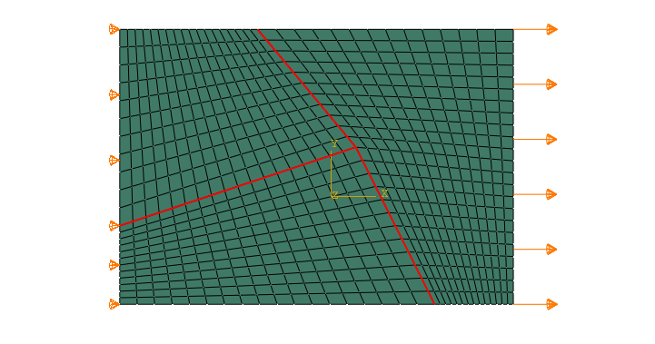
Assumptions:
• plane stress condition
• small strain theory
• elastic orthotropy of grains
Under plane stress conditions, such as in a shell element, only the values of $E_1$, $E_2$, $\nu_{12}$, $G_{12}$, $G_{13}$ and $G_{23}$ are required to define an orthotropic material. The shear moduli $G_{13}$ and $G_{23}$ are included because they may be required for modeling transverse shear deformation in a shell.
The Poisson's ratio $\nu_{21}$ is implicitly given as $\nu_{21} = (E_2/E_1)\nu_{12}$
Material parameters:
| $E_1$ | $E_2$ | $\nu_{12}$ | $G_{12}$ | $G_{13}$ | $G_{23}$ |
|---|---|---|---|---|---|
| $200$ | $100$ | $0.4$ | $50$ | $50$ | $50$ |
The stress-strain relations for the in-plane components of the stress and strain are of the form
$$\begin{bmatrix}\varepsilon _{11}\\\varepsilon _{22}\\\gamma _{12}\end{bmatrix}= \begin{bmatrix}1/E_1&-\nu_{12}/E_1&0\\ &1/E_2&0\\ sym& &1/G_{12}\end{bmatrix} \begin{bmatrix}\sigma _{11}\\\sigma _{22}\\\sigma _{12}\end{bmatrix}$$