Finite Element Method (FEM)
The Finite Element Method (FEM) is a powerful numerical technique used in continuum mechanics to analyze and simulate the behavior of deformable materials, structures, and other physical systems.
The basic finite element equation is based on a virtual work principle
$$\int_{\Omega}\ss \cdot \delta \D dV + \int_{\Omega} \rho \ddot{\u} \delta \v dV = \int_{\partial\Omega}\t \delta \v dS + \int_{\Omega} \f \delta \v dV$$where
• $\rho$ is the density
• $\rho$ known stress vector $\ss \n = \t$
• $\ss$ is the "true" Cauchy stress tensor
• $\f$ is a vector of body forces
• $\delta \v$ is the virtual displacement vector
• $\delta \D$ is the virtual strain rate (the virtual rate of deformation)
The above qutions also called the weak formulation is a re-formulation of the original PDE (Strong form).
The discretized equilibrium equations for the finite element method are
$$[\M] [\ddot{\u}] + [\I] = [\P]$$where
• $[\M]$ is the consistent mass matrix
• $[\P]$ is the external force vector
• $[\I]$ is the internal force vector (created by stresses in the elements)
The main steps of FEM:
Discretization The first step is to discretize the continuous domain (the object or structure under consideration) into smaller, finite elements. These elements can be triangles, quadrilaterals, tetrahedra, or other shapes depending on the dimensionality of the problem (2D or 3D). Nodes are placed at the vertices of these elements.
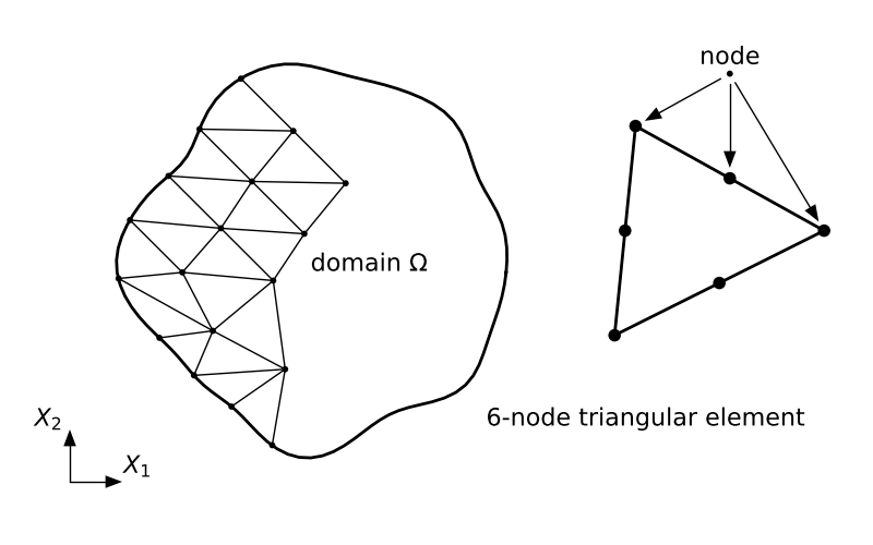
In FEM, the domain is understood as divided into a finite number of disjoint subdomains called finite elements. The way the elements are defined should ensure their simple and convenient geometrical shape so that approximating functions can be defined in a relatively straightforward way within each of the elements. For a 2D domain, this could be e.g. triangles or tetragons while for a 3D domain one may consider e.g. tetrahedra or other simple polyhedra able to completely fill the domain.
The domain $\Omega$ is divided into $E$ finite elements $\Omega_e, e = 1, 2, . . . , E$
$${\Omega} = \sum_{e=1}^{E} \Omega_e$$Upon such assumptions integrals over $\Omega$ can be expressed as sums of integrals over particular element domains.
$$\int_{\Omega} (\cdot) dV = \sum_{e=1}^{E} \int_{\Omega_e} (\cdot)dV$$Interpolation The next step involves interpolating the field variables (such as displacement, stress, or temperature) within each element. Typically, shape functions or basis functions are used to approximate these variables. This allows us to express the behavior within each element in terms of the values at the element's nodes.
$$u(\x) = \phi_i q_i, \quad i = 1, 2, ..., N$$One may assume that $N$ is the number of nodes $\x_i$in the FEM model and require that the coefficients $q_i$ equal values of the approximated field at corresponding nodes, respectively, i.e.
$$\u(\x_i) = q_i$$The so-defined coefficients $q_i$ are usually called nodal parameters.
Assembly The system of equations of FEM is assembled by combining the contributions from all elements. This is done by enforcing continuity conditions at the shared nodes of elements.
Boundary Conditions Essential and natural boundary conditions are applied to the system. Essential boundary conditions (e.g., fixed displacements, temperature) are enforced by directly modifying the equations, while natural boundary conditions (e.g., applied forces) are included in the force or load vector.
Solution The system of equations, which is often large and sparse, is solved using numerical methods, such as direct solvers or iterative techniques. The solution provides the values of the field variables (e.g., displacements, stresses) throughout the domain.
Implicit and explicit finite element analysis
Implicit and explicit finite element analysis (FEA) are two different approaches to solving finite element models of physical systems. They differ in their treatment of time integration and are suited for different types of problems:
Implicit solution of static equalibrium
Static equilibirum means that the inertia forces vary slowly, or are constant with time. This implies that
$$[\M] [\ddot{\u}] \approx [0]$$The implicit procedure is effective when the analysis ca be performed in realtively few time (load) increments
The Newton metod is usedd to solve for static equilibirum. Assuming that the we know the solution at iteration (i), $[\u]_i$ a Taylor series expansion gives
$$- [\I] + \left( \pp{[\P]}{[\u]} - \pp{[\I]}{[\u]} \right)[\c] + ... = 0$$where $[\c]$ is the correction to the solution $\Delta [\u]_{i+1} = \Delta [\u]_i + [\c]_i$.
The above equation can be rewritten as
$$[\c] = [\P] - [\I]$$where
$$= \pp{[\P]}{[\u]} - \pp{[\I]}{[\u]}$$is the system's tangent stiffness, or Jacobian matrix. Iterations are repeated in each increament unitil convergence is achived which means that the force equilibrium is satisfied.
Implicit:
• Solve for $t + \Delta t$ using the state at $t$ and $t + \Delta t$.
• The Newton method is used.
• Take an initial guess and iterate to convergence.
• This results in solving a linear system of equations.
• It is very accurate.
• This method allows for the use of relatively large time steps.
Explicit solution of static equalibrium
The explicit procedure performs the analysis using a large number of inexpensive saml time (load) increments. In the explicit procedure a diagonal mass matrix is used for efficiency. Thus the nodel accelerations can be obtained easily:
$$[\ddot \u] = [\M]^{-1} \cdot ([\P]-[\I])$$The central difference integration rule is used to update the velocities and displacment. The central difference integration rule is only conditionally stabe, that is the solution becomes unstable and diverges repidly if the time increment is too big
Explicit:
• Solve for the state at $t + \Delta t$ using the state at $t$.
• Requires the use of very small time steps.
• This method is very robust.
• There is no need for convergence checks.
• Solves directly for incremental displacement.
The Abaqus products
Abaqus/Standard is a general-purpose analysis product that can solve a wide range of linear and nonlinear problems involving the static, dynamic, thermal, electrical, and electromagnetic response of components. This product is discussed in detail in this guide. Abaqus/Standard solves a system of equations implicitly at each solution increment.
Abaqus/Explicit is a special-purpose analysis product that uses an explicit dynamic finite element formulation. It is suitable for modeling brief, transient dynamic events, such as impact and blast problems, and is also very efficient for highly nonlinear problems involving changing contact conditions, such as forming simulations. Abaqus/Explicit is discussed in detail in this guide.
Example 2: Lagrangian and Eulerian analysis of compression test
The goal of this example is to demonstrate the difference between two methods of describing motion in Abaqus. The analysis examines the compression of a thin plate under plane strain conditions. The plate is clamped between two rigid parts and is modeled as an elastic-plastic material.
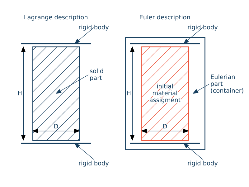
In the first model, the Lagrangian approach is used, where the material points remain fixed within the deforming body. In the second model, the Eulerian approach is applied, where the material flows through a fixed computational mesh, with the initial material assignment specified.
| Young's modulus | 200e3 [MPa] |
|---|---|
| Poisson ratio | 0.3 [-] |
| Plasticity | [100 MPa, 0],[ 200MPa 1] |
| Density | 7000e-12 [$t/mm^3$] |
| height H | 50 [mm] |
| width D | 20 [mm] |
| friction coefficient | 0.5 [-] |
| Time period | 0.0001 [s] |
| Velocity | 100000 [mm/s] |