Continuum Mechanics - in a nutshell
Continuum mechanics studies the response of materials to different loading conditions. Its subject matter can be divided into two main parts: (1) general principles common to all media and (2) constitutive equations defining idealized materials. The general principles are axioms considered to be self-evident from our experience with the physical world, such as conservation of mass; the balance of linear momentum, moment of momentum, and energy.
Notation
• index notation
• matrix motation
• absolute notation
Examples of notation and summation convention
• scalar
$$\alpha, \quad \alpha, \quad \alpha$$• vector
$$v_i, \quad \vc{v_1}{v_2}{v_3}, \quad \boldsymbol{v}$$• second order tensor
$$A_{ij}, \quad [A] = \mat{A_{11}}{A_{12}}{A_{13}}{A_{21}}{A_{22}}{A_{23}}{A_{31}}{A_{32}}{A_{33}}, \quad \A$$• dot product of two vectors
$$\alpha = v_iw_i, \quad \alpha = [v]^T \cdot [w] = \vr{v_1}{v_2}{v_3} \cdot \vc{w_1}{w_2}{w_3}, \quad \v \cdot \w$$• tensor product of two vectors
$$A_{ij} = v_iw_j, \quad [\A] = [v] \cdot [w]^T = \vc{v_1}{v_2}{v_3} \cdot \vr{w_1}{w_2}{w_3}, \quad \v \otimes \w$$• gradient of vector
$$h_{ij}=\pp{u_i}{x_j}=u_{i,j}, \quad [h]=\mat{\pp{u_1}{x_1}}{\pp{u_1}{x_2}}{\pp{u_1}{x_3}}{\pp{u_2}{x_1}}{\pp{u_2}{x_2}}{\pp{u_2}{x_3}}{\pp{u_3}{x_1}}{\pp{u_2}{x_3}}{\pp{u_3}{x_3}}, \quad \h = \u \otimes \nabla$$Deformable body
A deformable body is a physical body that deforms, meaning it changes its shape or volume under the influence of an external force.
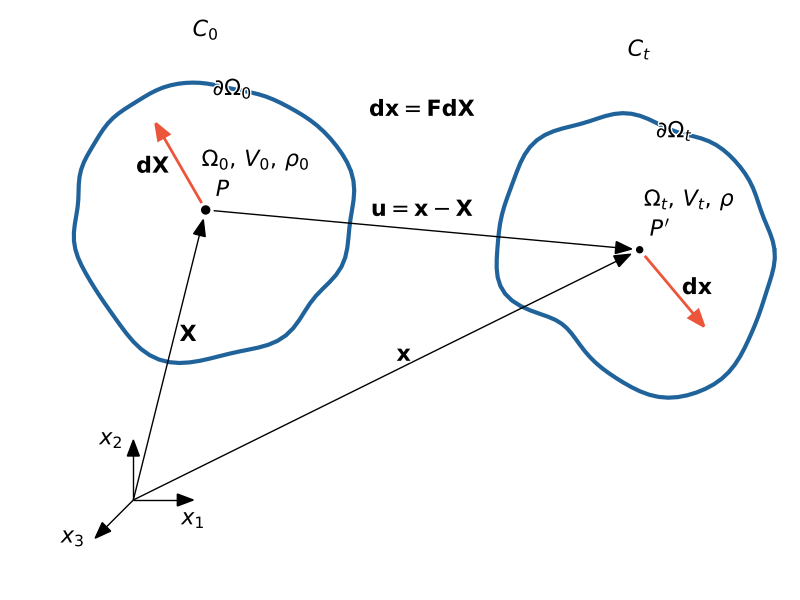
We distinguish two configurations - the initial configuration $C_0$ and the current configuration $C_t$. The body occupies a specific region at any moment of time $\Omega$. The body has it own volume $V$ and density $\rho$. $\X$ - represents the initial or reference position of the material point, whereas - $\x$ - represents its the current or deformed position. The displacement vector $\u$ represents the change in position of a material point within a deformable body as it undergoes deformation. The deformation gradient $\F$ describes how material element $\d\X$ within a deformable body have changed from their original (inital) configuration to their current deformed state $\d\x$.
Descritpion of motion
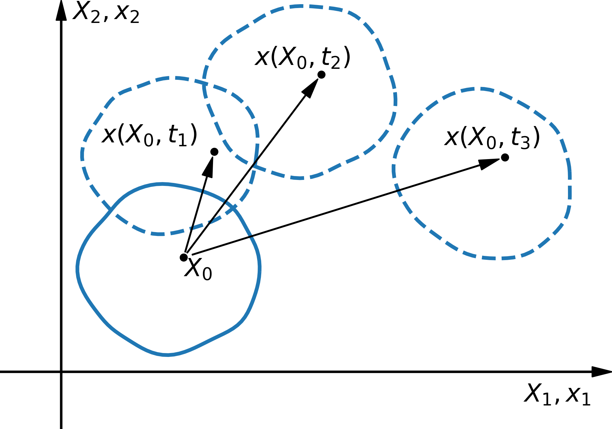
• material description (Lagrange descripition)
In the Lagrange description, the material is tracked individually as it deforms. It focuses on observing the properties and motion of specific material particles or elements as they move through space and change their positions. This approach is highly suited for studying the internal behavior of materials and how they evolve over time.
• spatial description (Euler description)
In the Eulerian description, the analysis is conducted from a fixed point of reference in space, often referred to as a control volume or grid. Instead of tracking individual material particles, it focuses on the properties and behaviors of the material within specific regions of space. This approach is well-suited for studying the flow of materials, such as fluids or gase
$$\X = \X(\x,t)$$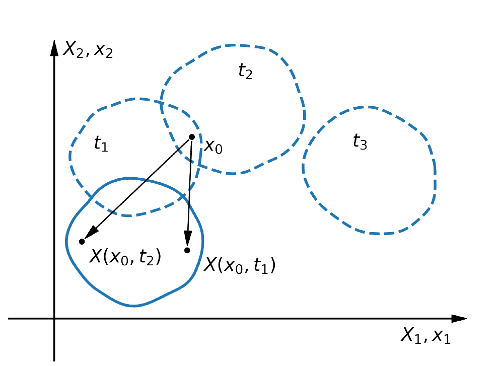
Conservation of mass, continuity equation
The principle of mass conservation dictates that mass remains constant throughout motion and deformation. In other words, both the entire body and its constituent parts maintain their original mass. Consequently, at any given moment in time,
$$m = \int_{\Omega_t} \rho(\x,t) \,dV_t = \mathrm{const}.$$The widely recognized differential and local form of mass conservation law is often referred to as the continuity equation
$$\dot{\rho} + \rho v_{i,i} = 0, \quad \dot{\rho} + \rho \div \v = 0$$Convervation of momentum, equation of motion
The momentum conservation law is essentially an extension of Newton's second law of motion to encompass deformable continua. In accordance with Newton's law, any alteration in the momentum of an object (or its constituent part) is equivalent to the cumulative effect of all forces exerted on that object (or part).
$$\dot{P} = F$$Applying Newton's second law of dynamics to a deformable body leads to
$$\sigma_{ji,j} + b_i = \rho \ddot{u}_i, \quad \div \ss^T + \b = \rho \ddot{\u}$$Angular Momentum Conservation Law
The angular momentum conservation law is again a generalization of the Newton’s second law of motion. It says that any change in angular momentum (also called moment of momentum) of a body (or its part) equals the sum of all moments of forces acting on the body (or its part)
$$\dot{K}_0 = M_0$$ $$\sigma_{ji} \epsilon_{ijk} = 0 \rightarrow \sigma_{ij} = \sigma_{ji}, \boldsymbol{\sigma} = \boldsymbol{\sigma}^T$$Geometric equations
Geometric equations refer to the connections between elements of the strain tensor and elements of the displacement vector. Their form depends on the strain measure we used.
For example:
$$\varepsilon_{ij} = \cfrac{1}{2}(u_{i,j} + u_{j,i} - u_{k,i}u_{k,j}), \quad \boldsymbol{\varepsilon} = \cfrac{1}{2}(\h + \h^T - \h^T\h), \quad \h = \u \otimes \nabla$$Constitutive equations
The equations listed in the preceding sections apply to any solid or fluid that deforms under the action of external forces. They do not, by themselves, have a unique solution, however, because the deformations are not related in any way to internal forces. The governing equations are completed by constitutive laws that provide the missing connection. Unlike deformation measures; kinetics; and conservation laws, a constitutive law cannot be calculated or predicted
In general form, the constitutive equations can be written as
$$f(\sigma_{ij}, \varepsilon_{ij}, \rho, t, ..., ) = 0$$Heat equation
Heat is another form of energy accumulated and transferred in material. The necessary condition for heat transfer between two interacting systems (bodies or subdomains in a body) is a temperature difference between the systems. There are various forms of heat energy transfer, such as conduction, convection or radiation. In mechanical systems, these processes are usually accompanied by a heat production due to inelastic deformation. Besides, in a body subject to temperature changes, thermal stresses and strains appear.
$$\rho c \dot{T} = - q_{i,i} + \rho r, \quad q_i = -\lambda_{ij} T_{,j},$$where $q_i$ is the heat flux, $c$ - specific heat, $r$ - internal heat sources.
Fundamental system of equations
The fundamental system of equations in continuum mechanics consists of differential equations accompanied by initial and boundary conditions.
• continuity equation
$$\dot{\rho} + \rho v_{i,i} = 0$$• equation of motion
$$\sigma_{ji,j} + b_i = \rho \ddot{u}_i$$• geometric equations
$$\varepsilon_{ij} = \cfrac{1}{2}(u_{i,j} + u_{j,i} - u_{k,i}u_{k,j})$$• constitutive equations
$$f(\sigma_{ij}, \varepsilon_{ij}, \rho, t, ..., ) = 0$$• heat equation, the law of conduction (constitutive law of heat flow)
$$\rho c \dot{T} = - q_{i,i} + \rho r, \quad q_i = -\lambda_{ij} T_{,j}$$Gradients in all the above equations are understood as partial derivatives with respect to coordinates in the current configuration $C_t$ and the time derivatives as material derivatives.
The necessary condition for existence of the solution is a consistent set of initial and boundary conditions for the unknown fields. The initial conditions have the following form
$$\rho(\x,0) = \rho^0(\x), \,\u(\x,0) = \u^0(\x), \,\v(\x,0) = \v^0(\x), \, \ss(\x,0) = \ss^0(\x)$$The boundary conditions (BC) imposed on the surface $\partial\Omega$ have two basic forms:
• kinematic (Dirichlet) BC, $\u = \hat{\u}(\x,t)$
• dynamic (Neumann) BC, $\ss\n = \hat{\t}(\x,t)$
To determine the temperature field from the heat equation, it is necessary to account for initial and boundary conditions. The initial condition establishes the initial temperature distribution
$$T(\x,0) = T^0(\x)$$The boundary conditions may imposed on
• the temperature distribution $T = \hat{T}(\x,t)$
• the heat flux distribution $\q= \hat{q}(\x,t)$
Thermomechanical couplings
• influence of geometry changes on the temperature field
• heat generation due to inelastic deformations
• variations in material constants due to temperature
• thermal expansion, expansion of materials under thermal conditions
• -
Abaqus
What is Abaqus?
Abaqus is a suite of powerful engineering simulation programs, based on the finite element method, that can solve problems ranging from relatively simple linear analyses to the most challenging nonlinear simulations. Abaqus contains an extensive library of elements that can model virtually any geometry. It has an equally extensive list of material models that can simulate the behavior of most typical engineering materials including metals, rubber, polymers, composites, reinforced concrete, crushable and resilient foams, and geotechnical materials such as soils and rock.
How to install Abaqus?
Abaqus Learning Edition
The Abaqus Learning Edition is available free of charge to anyone wishing to get started with Abaqus.
The Abaqus Learning Edition is available on Windows platform only and supports structural models up to 1000 nodes. The full documentation collection in HTML format makes this the perfect Abaqus learning tool. You can download the ABAQUS Learning Edition free of charge from the SIMULIA Community.
IPPT PAN license
Download the Abaqus (full version) from IPPT PAN website.
http://dsk.ippt.pan.pl/
index.php/oprogramowanie/abaqus
You need to have acces to the IPPT PAN internal network. To use abaqus from your home you must have access to a license using a VPN.
The Abaqus product suite consists of five core software products
Computer-Aided Engineering It is a software application used for both the modeling and analysis.
Abaqus/Standard a general-purpose Finite-Element analyzer that employs implicit integration scheme (traditional).
Abaqus/Explicit a special-purpose Finite-Element analyzer that employs explicit integration scheme to solve highly nonlinear systems.
Abaqus/CFD a Computational Fluid Dynamics software application which provides advanced computational fluid dynamics capabilities..
Abaqus/Electromagnetic a computational electromagnetics software application which solves advanced computational electromagnetic problems
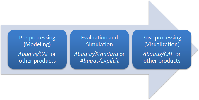
Workflow
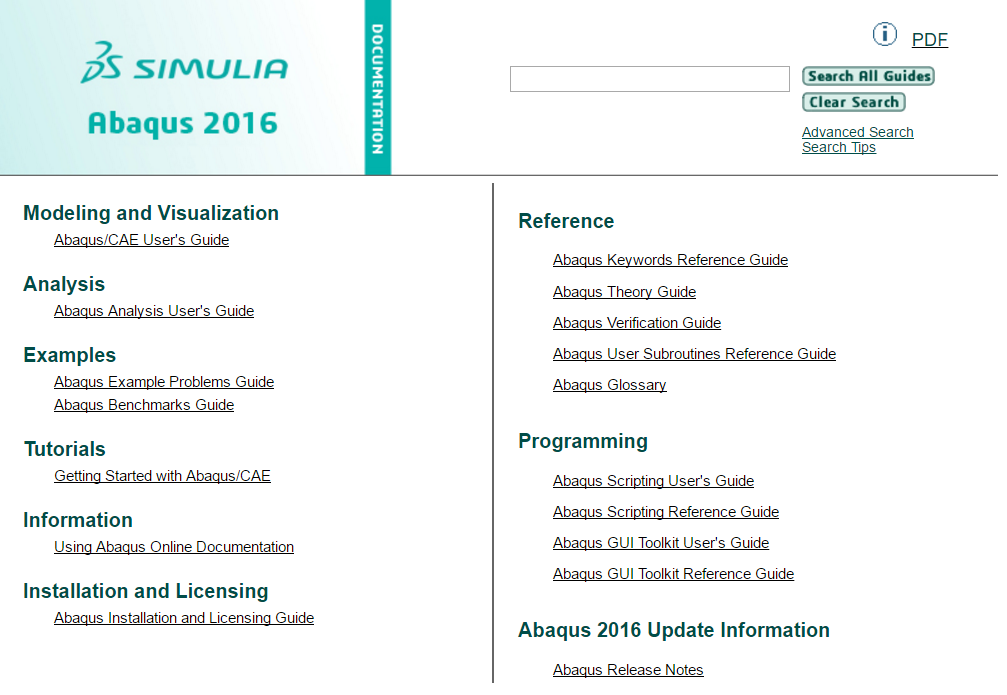
Documentation
Abaqus/CAE modules
Part - Sketch a two-dimensional profile and create a part representing the object.
Property - Define the material properties and other section properties of the part.
Assembly - Assemble the model.
Step - Configure the analysis procedure and output requests.
Load - Apply loads and boundary conditions to the parts.
Mesh - Mesh the parts.
Job - Create a job and submit it for analysis.
Visualization - View the results of the analysis.
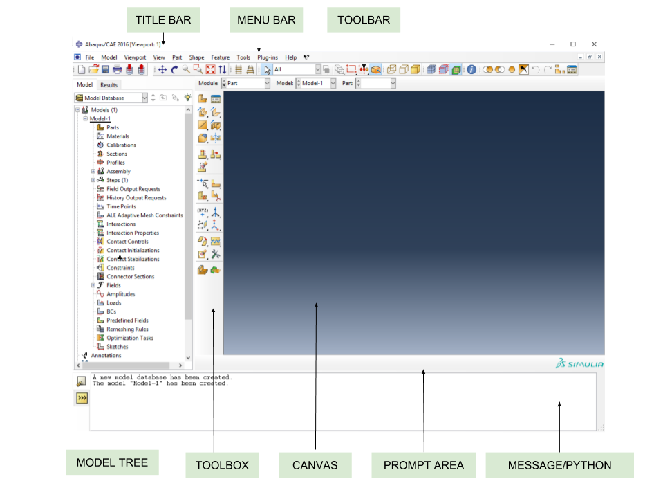
ABAQUS CAE
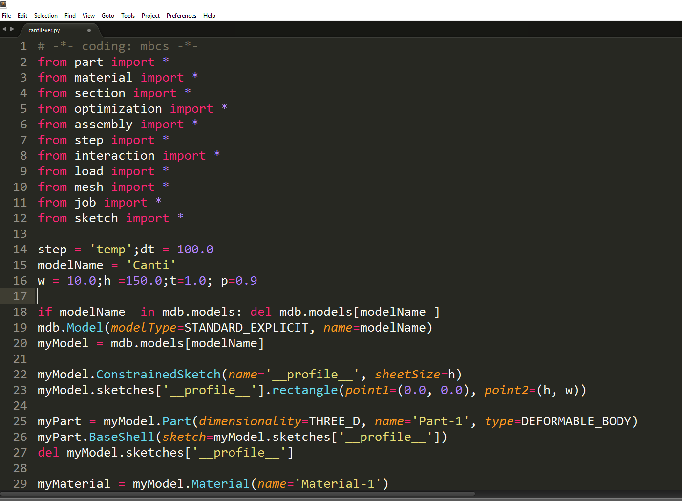
Python Scripts for Abaqus
Python scripts let you accomplish tasks in Abaqus that would be time consuming or practically impossible in the GUI (Abaqus/CAE). Using a script you can automate a repetitive task, vary parameters of a simulation as part of an optimization study, extract information from large output databases.
Input file
The input file is the means of communication between the preprocessor, usually ABAQUS/CAE, and the analysis product, ABAQUS/Standard. It contains a complete description of the numerical model. The input file is a text file that has an intuitive, keyword-based format, so it is easy to modify using a text editor if necessary; if a preprocessor such as ABAQUS/CAE is used, modifications should be made using it. Indeed, small analyses can be specified easily by typing the input file directly.
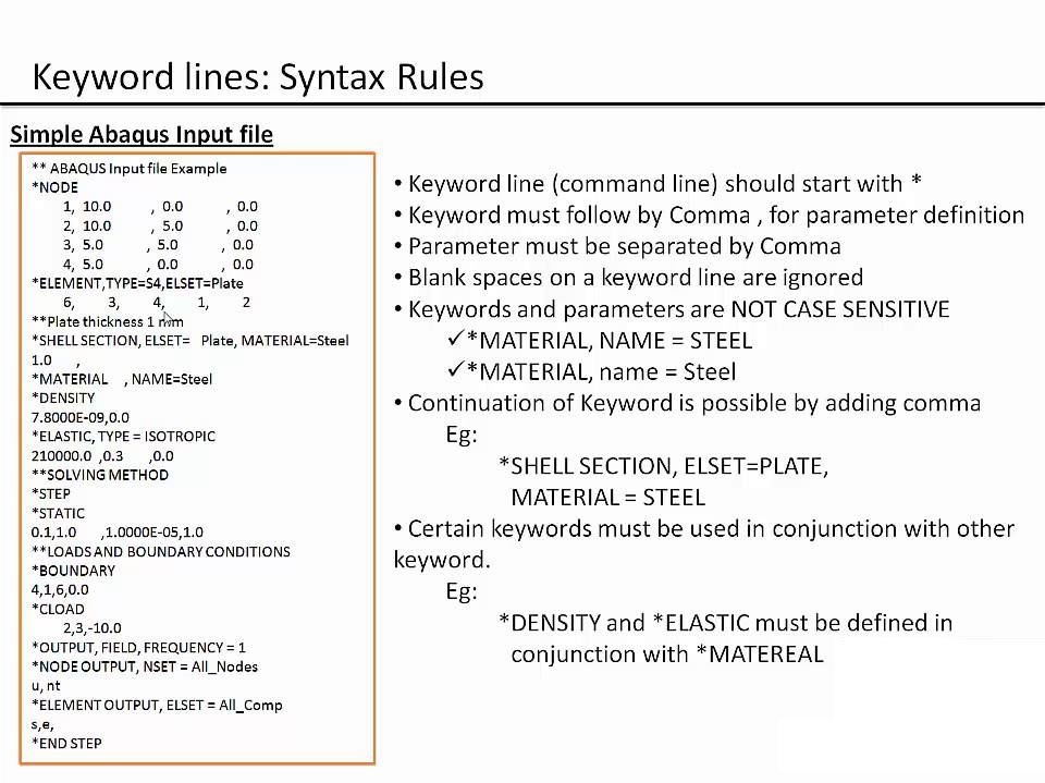
The input file is composed of a number of option blocks that contain data describing a part of the model. Each option block begins with a keyword line, which is usually followed by one or more data lines. These lines cannot exceed 256 characters.
Units
Before starting to define any model, you need to decide which system of units you will use. ABAQUS has no built-in system of units.
| Quantity | SI | SI (mm) |
|---|---|---|
| Length | m | mm |
| Force | N | N |
| Mass | kg | tonne (10$^{3}$kg) |
| Time | s | s |
| Stress | Pa (N/m$^2$) | MPa (N/mm$^2$) |
| Energy | J | mJ (10$^{-3}$J) |
| Density | kg/m$^3$ | tonne/mm$^3$ |
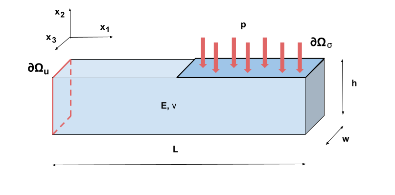
"Hello world" with Abaqus
Analysis of deformation of a simply supported beam subjected to continuous loading
Assumptions:
• small strain theory $\F \approx \I, \quad \rho \approx \rho_0$
• quasi static process $\ddot{\u} \approx 0$
• lack of body forces $\b = 0$
• linear isotropic elastic material $\ss = \C \ee$, $E$ - Young's modulus, $\nu$ - Poisson ratio
A complete set of equations describing the problem is as follows
$$\left\{\begin{array}{ll} \sigma_{ij,j} = 0\\ \varepsilon_{ij} = \cfrac{1}{2}(u_{i,j}+ u_{j,i})\\ \sigma_{ij} = \cfrac{E}{2(1+\nu)}\varepsilon_{ij} + \cfrac{Ev}{(1+\nu)(1-2\nu)} \varepsilon_{kk}\delta_{ij} \end{array} \right.$$The are two types of boundary conditions:
$$\u(\x) = \hat{\u}(\x) = 0, \quad \x \in \partial\Omega_u$$ $$\ss\n(\x) = \hat{\t}(\x) = p \I \e_2 = p \e_2, \quad \x \in \partial\Omega_{\sigma}$$